9 Autonomous Equations and Stability

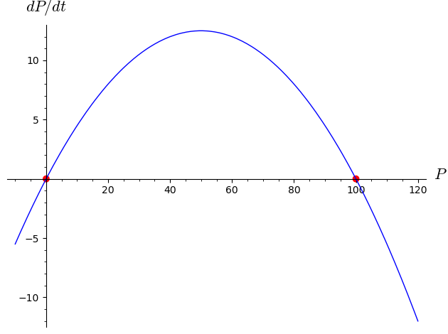
SageMath Spotlight

Plotting phase portraits:
- plot(f(y), (y, y_min, y_max), axes_labels=['$y$', '$dy/dt$'])

9.1 Autonomous Differential Equations

In Chapter 8, we explored differential equations where the rate of change depended on both time $t$ and the state $y$. However, many physical and biological systems are modeled by rules that do not explicitly depend on when the process is happening, but only on the current state of the system.

Autonomous Differential Equations

A first-order differential equation is autonomous if the independent variable¹ does not explicitly appear on the right-hand side. These take the form: \[ \frac{\mathop{}\!\mathrm{d}y}{\mathop{}\!\mathrm{d}t} = f(y). \]

For example, both unconstrained population growth (Example 7.4) and logistic growth (Example 8.5) are autonomous equations—the growth rate depends entirely on the current population size $P$, regardless of what year it is.

Stability of Equilibrium Solutions

Because $\frac{\mathop{}\!\mathrm{d}y}{\mathop{}\!\mathrm{d}t}$ depends only on $y$, we can understand the long-term behavior of the system by graphing the rate of change $\frac{\mathop{}\!\mathrm{d}y}{\mathop{}\!\mathrm{d}t}$ against the state variable $y$: a phase portrait. From here, we can analyze the equilibrium solutions (where $f(y) = 0$) to qualitatively determine asymptotic behavior of the system.

Recall that, if $y_0$ is a value such that $f(y_0)=0$, then trajectories beginning at $y_0$ satisfy $\frac{\mathop{}\!\mathrm{d}y}{\mathop{}\!\mathrm{d}t} = 0$ and the system never changes. But what happens if the system is pushed slightly away from $y_0$? The sign of $f(y)$ tells us exactly how the system reacts:

If $f(y) > 0$, then $y(t)$ is increasing (moving to the right on a phase line).
If $f(y) < 0$, then $y(t)$ is decreasing (moving to the left on a phase line).

Based on this, every equilibrium point falls into one of three stability classifications:

Stable: The function $f(y)$ changes from positive to negative at the equilibrium. If the system is perturbed, the rate of change forces it back toward the equilibrium.
Unstable: The function $f(y)$ changes from negative to positive at the equilibrium. If the system is perturbed, it will move further and further away.
Semistable: The function $f(y)$ touches the axis but does not change sign (e.g., positive on both sides). The system will return to the equilibrium from one direction, but flee from it in the other.

Example 9.1 (Phase Portrait of the Logistic Model) Recall the logistic population model (Example 8.5): \[ \frac{\mathop{}\!\mathrm{d}P}{\mathop{}\!\mathrm{d}t} = k P \left(1 - \frac{P}{M}\right). \] As before, take $k = 0.5$ and $M = 100$. The phase portrait is a downward-opening parabola:

var('P')
rate_plot = plot(0.5 * P * (1 - P/100), (P, -10, 120), axes_labels=['$P$', '$dP/dt$'])
equilibria = point([(0,0), (100,0)], color='red', size=50)
show(rate_plot + equilibria)

We can classify our two equilibrium solutions as follows:

At $P = 0$: To the right of zero, the parabola is above the axis ($\frac{\mathop{}\!\mathrm{d}P}{\mathop{}\!\mathrm{d}t} > 0$). This means a small initial population will grow, moving away from zero. Similarly, negative initial values will become more negative and move away from the steady state (even if negative population does not make sense). Thus, $P=0$ is an unstable equilibrium.
At $P = 100$: If $P$ is slightly less than $M=100$, $\frac{\mathop{}\!\mathrm{d}P}{\mathop{}\!\mathrm{d}t} > 0$ and the population grows toward $M$. If $P$ is slightly greater than $M$, the parabola dips below the axis, so $\frac{\mathop{}\!\mathrm{d}P}{\mathop{}\!\mathrm{d}t} < 0$ (population shrinks toward $M$). Because trajectories from both sides point toward $M$, $P=M$ is a stable equilibrium.

Example 9.2 (A Semistable Equilibrium) Consider the autonomous equation: \[ \frac{\mathop{}\!\mathrm{d}y}{\mathop{}\!\mathrm{d}t} = (y - 2)^2. \] Setting $f(y) = 0$ yields a single equilibrium solution at $y = 2$.

var('y')
rate_plot = plot((y-2)^2, (y, -0.25, 4))
equilibrium = point([(2,0)], color='red', size=50)
show(rate_plot + equilibrium, axes_labels=['$y$', '$dy/dt$'])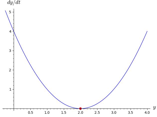

However, because $(y-2)^2$ is always positive (except exactly at $y=2$), the rate of change $\frac{\mathop{}\!\mathrm{d}y}{\mathop{}\!\mathrm{d}t}$ is positive on both sides of the equilibrium!

If $y < 2$, $\frac{\mathop{}\!\mathrm{d}y}{\mathop{}\!\mathrm{d}t} > 0$, so the solution grows toward $y=2$.
If $y > 2$, $\frac{\mathop{}\!\mathrm{d}y}{\mathop{}\!\mathrm{d}t} > 0$, so the solution continues to grow away from $y=2$.

Because it attracts from below but repels from above, $y=2$ is a semistable equilibrium. We conclude by considering the slope field associated to this differential equation, to see how it leads to the same conclusion:

var('t y')
f = (y-2)^2
slope_field = plot_slope_field(f, (t, -1, 3.5), (y, -0.25, 4), color='gray')
flow_lines = streamline_plot(f, (t, -1, 3.5), (y, -0.25, 4), color='blue', density=0.3)
equilibrium = plot(2, (t, -1, 3.5), color='red', linestyle='--')
show(slope_field + flow_lines + equilibrium, axes_labels=['$t$', '$y$'])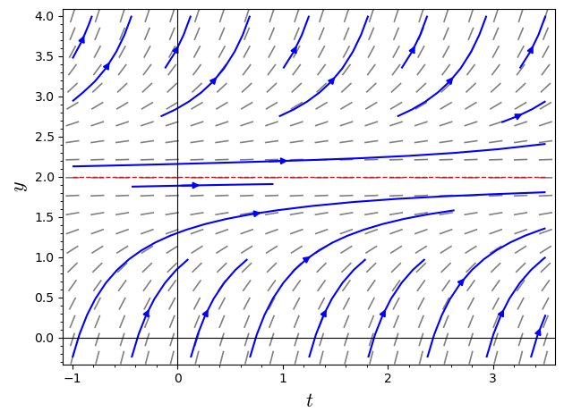

Often the independent variable is time $t$; these autonomous equations are also called time-independent.↩︎