var('x y')
f = x^2+y^2
print("The partial derivative with respect to x is", diff(f,x))The partial derivative with respect to x is 2*xSageMath Spotlight
diff(f, x)diff(f, x, y)When moving from functions of a single variable to functions of two or more variables, generalizing the concept of differentiation takes careful consideration. Fundamentally, derivatives ask about instantaneous rates of change: “How do these quantities change with respect to each other?” With functions of only one real variable, \(y = f(x)\), there is only one way the function can vary (albeit as \(x\) grows or shrinks). Now, instead of simply asking “how does the function change as we move along the \(x\)-axis?” we now have to specify a direction of travel.
The simplest directions to consider are parallel to the coordinate axes. This gives rise to the partial derivative (Stewart et al. 2020, 14.3, pp. 962).
If \(z = f(x,y)\), the partial derivative of \(f\) with respect to \(x\) at a point \((x_0, y_0)\) is given by: \[ \left[ \frac{\mathop{}\!\partial f}{\mathop{}\!\partial x} \right]_{(x_0,y_0)} \coloneqq \lim_{h \to 0} \frac{f(x_0 + h, y_0) - f(x_0, y_0)}{h}. \tag{15.1}\] In other words, we hold \(y\) constant (\(y = y_0\)) and take the standard single-variable derivative with respect to \(x\). Similarly, the partial derivative with respect to \(y\) holds \(x\) constant: \[ \left[ \frac{\mathop{}\!\partial f}{\mathop{}\!\partial y} \right]_{(x_0,y_0)} \coloneqq \lim_{h \to 0} \frac{f(x_0, y_0 + h) - f(x_0, y_0)}{h}. \tag{15.2}\] We will often use the more compact subscript notation: \[ f_x(x_0,y_0) \coloneqq \left[ \frac{\mathop{}\!\partial f}{\mathop{}\!\partial x} \right]_{(x_0,y_0)} \quad \text{and} \quad f_y(x_0,y_0) \coloneqq \left[ \frac{\mathop{}\!\partial f}{\mathop{}\!\partial y} \right]_{(x_0,y_0)}. \]
Just as with single-variable derivatives, once we learn to differentiate at a point, we can differentiate a function \(f\) to obtain another function \(f_x\) (or \(f_y\)) whose value at each point describes the partial derivative of \(f\) at the same point.
To compute \(f_x\), we treat \(y\) as a constant and apply the usual derivative rules.
Example 15.1 (\(f(x,y) = x^2+y^2\)) To find the partial derivative in \(x\) from the definition, we compute \[ \begin{aligned} f_x & = \lim_{h \to 0} \frac{f(x + h, y) - f(x, y)}{h} \\ & = \lim_{h \to 0} \frac{\left( (x+h)^2+y^2 \right) - \left( x^2+y^2 \right)}{h} \\ & = \lim_{h \to 0} \frac{\left( x^2+2xh+h^2+y^2 \right) - \left( x^2+y^2 \right)}{h} \\ & = \lim_{h \to 0} \frac{2xh+h^2}{h} \\ & = \lim_{h \to 0} 2x+h = 2x. \\ \end{aligned} \] This is rather cumbersome, so we remark at a much more straightforward route to the solution. If we temporarily consider \(x^2+y^2\) as a function only in \(x\), with \(y\) held as a constant, then we already know how to compute this derivative from Calculus I: \[ \frac{\mathop{}\!\partial }{\mathop{}\!\partial x} (x^2+y^2) = 2x + 0 = 2x. \] Since the term \(y^2\) is just a constant, it vanishes when we differentiate!
Similarly, to compute the partial derivative in \(y\), we treat \(x\) as a constant: \[ \frac{\mathop{}\!\partial }{\mathop{}\!\partial y} (x^2+y^2) = 0 + 2y = 2y. \]
We can check our work with Sage:
var('x y')
f = x^2+y^2
print("The partial derivative with respect to x is", diff(f,x))The partial derivative with respect to x is 2*xGeometrically, computing a partial derivative at a point is equivalent to slicing the surface with a vertical plane (either \(y = y_0\) or \(x = x_0\)) and finding the slope of the tangent line (with classic 1-variable calculus!) to the resulting 2D trace curve.
Example 15.2 (\(f(x,y) = x^4 + y^4 - 4xy\)) Returning to Example 14.3, suppose we want to find the slopes of the surface at the point \((x,y) = (\frac{1}{2}, 0)\). Note that the \(z\)-coordinate at this point is \(f(\frac{1}{2}, 0) = \frac{1}{16}\).
First, we compute the partial derivative functions using our standard Calculus I rules: \[ f_x(x,y) = 4x^3 - 4y \quad \text{and} \quad f_y(x,y) = 4y^3 - 4x. \] Evaluating these at the point \((\frac{1}{2}, 0)\) gives: \[ \begin{aligned} f_x\left(\tfrac{1}{2}, 0\right) & = 4\left(\tfrac{1}{8}\right) - 0 = \tfrac{1}{2} \\ f_y\left(\tfrac{1}{2}, 0\right) & = 0 - 4\left(\tfrac{1}{2}\right) = -2. \end{aligned} \]
Let’s visualize the surface alongside the two tangent lines passing through \((\frac{1}{2}, 0, \frac{1}{16})\): one pointing in the \(x\)-direction (red) with slope \(\frac{1}{2}\), and one pointing in the \(y\)-direction (blue) with slope \(-2\).
var('x y z t')
surface = implicit_plot3d(z==x^4 + y^4 - 4*x*y, (x, -2, 2), (y, -2, 2), (z, -2, 2), color='plum', opacity=0.6)
pt = point3d((1/2, 0, 1/16), color='black', size=30)
line_x = parametric_plot3d(
(1/2 + t, 0, 1/16 + (1/2)*t), (t, -1, 1),
color='red', thickness=3
)
line_y = parametric_plot3d(
(1/2, t, 1/16 - 2*t), (t, -1, 1),
color='blue', thickness=3
)
show(surface + pt + line_x + line_y)Moving forward, we will implicitly assume that the functions we study are differentiable—that is, that the limits Equation 15.1 and Equation 15.2 exist at all points in the function’s domain. In the multivariable context, this means that the surface is “smooth” and that these tangent lines do a good job of approximating the surface locally, without any sharp corners or cusps.
Just as we can differentiate equations implicitly (Section 1.2.6), given some algebraic relationship of many variables, we can compute partial derivatives without explicitly solving for \(z = f(x,y)\).
Example 15.3 Consider the hyperboloid of one sheet given by \(x^2 + y^2 - z^2 = 1\); we will compute the partial derivatives of this surface at the point \((x,y,z) = (\frac{7}{8}, \frac{1}{2}, \frac{1}{8})\). Instead of solving for \(z\) (which would yield \(z = \pm\sqrt{x^2+y^2-1}\), forcing us to deal with two separate branches and all sorts of nasty derivatives), we can treat \(z\) as an implicit function of \(x\) and \(y\).
To find \(\frac{\mathop{}\!\partial z}{\mathop{}\!\partial x}\), we differentiate both sides with respect to \(x\), treating \(y\) as a constant and remembering to use the chain rule on \(z = z(x,y)\):
\[ \begin{aligned} \frac{\mathop{}\!\partial }{\mathop{}\!\partial x}(x^2 + y^2 - z^2) &= \frac{\mathop{}\!\partial }{\mathop{}\!\partial x}(1) \\ 2x + 0 - 2z \frac{\mathop{}\!\partial z}{\mathop{}\!\partial x} &= 0 \\ 2z \frac{\mathop{}\!\partial z}{\mathop{}\!\partial x} &= 2x \\ \frac{\mathop{}\!\partial z}{\mathop{}\!\partial x} &= \frac{x}{z} \end{aligned} \]
Similarly, differentiating with respect to \(y\) yields \(\frac{\mathop{}\!\partial z}{\mathop{}\!\partial y} = \frac{y}{z}\). At the point of interest, we compute:
\[ \left[ \frac{\mathop{}\!\partial z}{\mathop{}\!\partial x} \right]_{(\frac{7}{8}, \frac{1}{2}, \frac{1}{8})} = 7 \quad \text{and} \quad \left[ \frac{\mathop{}\!\partial z}{\mathop{}\!\partial y} \right]_{(\frac{7}{8}, \frac{1}{2}, \frac{1}{8})} = 4 \]
var('x y z t')
surface = implicit_plot3d(x^2 + y^2 - z^2 == 1, (x, -2, 2), (y, -2, 2), (z, -2, 2), color='plum', opacity=0.6)
pt = point3d((7/8, 1/2, 1/8), color='black', size=30)
line_x = parametric_plot3d(
(7/8 + t, 1/2, 1/8 + 7*t), (t, -1/7, 1/7),
color='red', thickness=3
)
line_y = parametric_plot3d(
(7/8, 1/2 + t, 1/8 + 4*t), (t, -1/4, 1/4),
color='blue', thickness=3
)
show(surface + pt + line_x + line_y)The concept of a partial derivative extends naturally to functions of three or more variables! If \(w = f(x,y,z)\), we can compute \(f_x\), \(f_y\), and \(f_z\) by holding all other variables constant. For instance, if \(f(x,y,z) = x^2 y^3 e^z\), then \(f_y(x,y,z) = 3x^2 y^2 e^z\).
If we differentiate \(f(x,y)\), we get two new functions, \(f_x\) and \(f_y\). Since these are also functions of \(x\) and \(y\), we can differentiate them again to find the second partial derivatives of \(f\). Note that, a priori, this gives us four distinct functions: \[ f_{xx} \coloneqq \frac{\mathop{}\!\partial }{\mathop{}\!\partial x}\left(\frac{\mathop{}\!\partial f}{\mathop{}\!\partial x}\right), \quad f_{xy} \coloneqq \frac{\mathop{}\!\partial }{\mathop{}\!\partial y}\left(\frac{\mathop{}\!\partial f}{\mathop{}\!\partial x}\right), \quad f_{yx} \coloneqq \frac{\mathop{}\!\partial }{\mathop{}\!\partial x}\left(\frac{\mathop{}\!\partial f}{\mathop{}\!\partial y}\right), \quad f_{yy} \coloneqq \frac{\mathop{}\!\partial }{\mathop{}\!\partial y}\left(\frac{\mathop{}\!\partial f}{\mathop{}\!\partial y}\right). \]
The derivatives \(f_{xx}\) and \(f_{yy}\) are the pure second derivatives of \(f\); \(f_{xy}\) and \(f_{yx}\) are the mixed partial derivatives. Indeed, for most nice functions, the order in which we take mixed derivatives does not matter:
Clairaut’s Theorem (Stewart et al. 2020, 14.3, pp. 967)
Suppose \(f = f(x,y)\) is defined near \((x_0,y_0)\), and that \(f_{xy}\) and \(f_{yx}\) both exist and are continuous in this region. Then \(f_{xy}(x_0,y_0) = f_{yx}(x_0,y_0)\).
Example 15.4 Consider the mixed partial derivatives of \(f(x,y) = x^3 y^2 + \sin(xy)\). First, we find \(f_x\) and \(f_y\): \[ f_x(x,y) = 3x^2 y^2 + y\cos(xy) \quad \text{and} \quad f_y(x,y) = 2x^3 y + x\cos(xy) \] Now, differentiate \(f_x\) with respect to \(y\) (using the product rule): \[ \begin{aligned} f_{xy}(x,y) & = 6x^2 y + \left[ 1\cdot \cos(xy) + y(-\sin(xy)\cdot x) \right] \\ & = 6x^2 y + \cos(xy) - xy\sin(xy) \end{aligned} \] Lastly, we differentiate \(f_y\) with respect to \(x\): \[ \begin{aligned} f_{yx}(x,y) & = 6x^2 y + \left[ 1\cdot \cos(xy) + x(-\sin(xy)\cdot y) \right] \\ & = 6x^2 y + \cos(xy) - xy\sin(xy) \end{aligned} \] As Clairaut’s Theorem guarantees, we find that \(f_{xy} = f_{yx}\).
As before, we can check our work:
var('x y')
f = x^3 * y^2 + sin(x*y)
fxx = diff(f, x, x)
fxy = diff(f, x, y)
fyx = diff(f, y, x)
fyy = diff(f, y, y)
print("The pure second derivatives are", fxx, "and", fyy)
print("The mixed derivatives are", fxy, "and", fyx)The pure second derivatives are 6*x*y^2 - y^2*sin(x*y) and 2*x^3 - x^2*sin(x*y)
The mixed derivatives are 6*x^2*y - x*y*sin(x*y) + cos(x*y) and 6*x^2*y - x*y*sin(x*y) + cos(x*y)In Calculus I, we found local maximums and minimums by locating critical points: values of \(x\) where \(f'(x) = 0\). As we will see, we have a direct analogue for functions of two variables.
Theorem (Stewart et al. 2020, 14.7, pp. 1009)
Suppose \(f = f(x,y)\) is a differentiable function near the point \((x_0,y_0)\). If \(f\) has a local maximum or minimum at \((x_0,y_0)\), then \(f_x(x_0,y_0) = 0\) and \(f_y(x_0,y_0) = 0\).
We call any point where \(f_x = 0\) and \(f_y = 0\) simultaneously a critical point. Let’s examine our three examples from Chapter 14 to see this in action.
Example 15.5 (\(f(x,y) = x^2+y^2\)) For the paraboloid, we already found that \(f_x = 2x\) and \(f_y = 2y\), and so the only critical point is \((0,0)\). Since \(x^2+y^2 \ge 0\) for all real numbers, this point is a global minimum, aligning with our visual intuition of a bowl.
Example 15.6 (\(f(x,y) = \sin x + \cos y\)) Consider \(f(x,y) = \sin x + \cos y\), so that \(f_x = \cos x\) and \(f_y = - \sin y\). At the origin, we have \[ f_x(0,0) = 1 \quad \text{and} \quad f_y(0,0) = 0 \] Because \(f_x(0,0) \not = 0\), the origin cannot be a local max or min. Geometrically, moving in the positive \(x\)-direction from the origin yields an upward slope—in fact, a path of steepest ascent! However, if we check the point \((\tfrac{\pi}{2}, 0)\), then we have
\[ f_x\left(\tfrac{\pi}{2}, 0\right) = 0 \quad \text{and} \quad f_y\left(\tfrac{\pi}{2}, 0\right) = 0. \]
Both partial derivatives are zero, indicating a horizontal tangent plane. This point represents the top of one of our “hills”, a local maximum.
var('x y z t')
surface = plot3d(
sin(x) + cos(y), (x, -6, 6), (y, -6, 6),
color='lightblue', opacity=0.7
)
pt1 = point3d((0, 0, 1), color='black', size=50)
pt2 = point3d((pi/2, 0, 2), color='black', size=50)
line_x = parametric_plot3d(
(t, 0, 1+t), (t, -2, 2),
color='red', thickness=3
)
line_y = parametric_plot3d(
(0, t, 1), (t, -2, 2),
color='blue', thickness=3
)
show(surface + pt1 + line_x + line_y + pt2)Example 15.7 (\(f(x,y) = x^4 + y^4 - 4xy\)) Continuing Example 15.2, we will find all the critical points for \(f(x,y) = x^4 + y^4 - 4xy\). We need both partial derivatives, \[ f_x = 4x^3 - 4y \quad \text{and} \quad f_y = 4y^3 - 4x, \] to be zero simultaneously. We can visualize this by plotting the two curves \(f_x = 0\) (in red) and \(f_y = 0\) (in blue) on top of the level curves of the function:
var('x y')
f = x^4 + y^4 - 4*x*y
fx = diff(f,x)
fy = diff(f,y)
contours = contour_plot(
f, (x, -2, 2), (y, -2, 2),
contours=(-1.8, -1.2, -0.6, 0, 1, 2, 4, 8, 16), fill=False
)
fx_zero = implicit_plot(
fx == 0, (x, -2, 2), (y, -2, 2),
color='red', linewidth=3
)
fy_zero = implicit_plot(
fy == 0, (x, -2, 2), (y, -2, 2),
color='blue', linewidth=3
)
show(contours + fx_zero + fy_zero, figsize=6)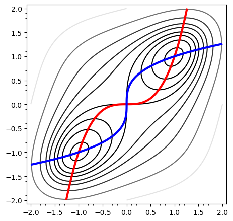
Critical points exist exactly where the red and blue curves intersect! Algebraically, we have:
flowchart LR
A("4x³ - 4y = 0 <br> 4y³ - 4x = 0")
A --> B("y = x³ <br> x = y³")
B --> C("x = (x³)³")
C --> D("x = 0, 1, -1")
D --> E("(x,y) = (0,0), (1,1), (-1,-1)"):::solution
B --> E
Looking at the contours and surface plots, we can see that \((1,1)\) and \((-1,-1)\) reside at the bottom of the two “legs” (we call them local minima). But what is happening at the origin?—this point is neither a min or a max!