curve = plot( x*e^x, (x, -5, 0.5), axes_labels=['$x$', '$y$'])
shaded_area = plot( x*e^x, (x, -5, 0), fill=True)
show(curve + shaded_area)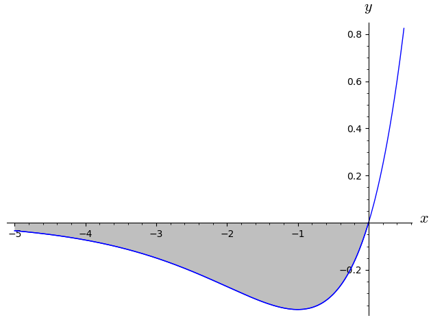
SageMath Spotlight
integral(f(x), x)integral(f(x), x, a, b)oo (it’s supposed to look like \(\infty\))Up to this point, our definition of the definite integral \(\int_a^b f(x) \mathop{}\!\mathrm{d}x\) has rested on two fundamental assumptions:
In many real-world applications—such as computing total work over infinite distances in physics, analyzing continuous probability distributions in statistics, or measuring long-term financial yield—we must relax these conditions. When an integral runs off to infinity or encounters a vertical asymptote, we call it an improper integral. The guiding principle for all improper integrals is simple: we replace the infinite or problematic point with a limit!
When the domain of integration extends indefinitely, we replace \(\infty\) or \(-\infty\) with a variable \(t\) which we then tend off to infinity. The book calls these Type 1 improper integrals (Stewart et al. 2020, 7.8, pp. 546), though we will not use this name:
Unbounded Domain
\[ \int_a^\infty f(x) \mathop{}\!\mathrm{d}x \coloneqq \lim_{t \to \infty} \int_a^t f(x) \mathop{}\!\mathrm{d}x \quad \text{and} \quad \int_{-\infty}^b f(x) \mathop{}\!\mathrm{d}x \coloneqq \lim_{t \to -\infty} \int_t^b f(x) \mathop{}\!\mathrm{d}x. \]
Example 6.1 (\(\int_{-\infty}^0 x e^x \mathop{}\!\mathrm{d}x\)) We begin by considering \(\int_t^0 x e^x \mathop{}\!\mathrm{d}x.\) Integrating by parts (\(u = x\) and \(\mathop{}\!\mathrm{d}v = e^x \mathop{}\!\mathrm{d}x\)), we have: \[ \int x e^x \mathop{}\!\mathrm{d}x = x e^x - e^x. \] We evaluate over the bounds \([t, 0]\): \[ \int_t^0 x e^x \mathop{}\!\mathrm{d}x = (0 \cdot e^0 - e^0) - (t e^t - e^t) = -1 - t e^t + e^t. \] Taking the limit as \(t \to -\infty\) requires using L’Hôpital’s rule on the \(t e^t\) term: \[ \lim_{t \to -\infty} t e^t = \lim_{t \to -\infty} \frac{t}{e^{-t}} = \lim_{t \to -\infty} \frac{1}{-e^{-t}} = 0, \] and so the integral converges: \[ \int_{-\infty}^0 x e^x \mathop{}\!\mathrm{d}x = \lim_{t \to -\infty} \int_t^0 x e^x \mathop{}\!\mathrm{d}x = -1 - 0 + 0 = -1. \] We conclude with a picture:
curve = plot( x*e^x, (x, -5, 0.5), axes_labels=['$x$', '$y$'])
shaded_area = plot( x*e^x, (x, -5, 0), fill=True)
show(curve + shaded_area)
If \(f(x)\) approaches \(\pm\infty\) at a point within or on the boundary of \([a, b]\), we cannot apply the Fundamental Theorem of Calculus directly. Instead, we approach the asymptote using a one-sided limit. The book calls these Type 2 improper integrals (Stewart et al. 2020, 7.8, pp. 546).
Unbounded Integrand at an Endpoint
If \(f(x)\) is continuous on \((a, b]\) but discontinuous at \(x = a\), we define: \[ \int_a^b f(x) \mathop{}\!\mathrm{d}x = \lim_{t \to a^+} \int_t^b f(x) \mathop{}\!\mathrm{d}x. \] If this limit exists as a finite number, we say the integral converges. Otherwise, it diverges.
Example 6.2 (\(\int_0^1 \frac{1}{\sqrt{x}} \mathop{}\!\mathrm{d}x\)) The function \(x^{-1/2}\) has a vertical asymptote at \(x = 0\). Replacing \(0\) with \(t > 0\) gives: \[ \begin{aligned} \int_0^1 \frac{1}{\sqrt{x}} \mathop{}\!\mathrm{d}x & = \lim_{t \to 0^+} \int_t^1 x^{-1/2} \mathop{}\!\mathrm{d}x \\ & = \lim_{t \to 0^+} \left[ 2\sqrt{x} \right]_t^1 \\ & = \lim_{t \to 0^+} \left( 2\sqrt{1} - 2\sqrt{t} \right) = 2 - 0 = 2. \end{aligned} \] The integral converges to \(2\). Even though the curve grows infinitely tall at \(x = 0\), it thins out quickly enough to enclose a finite area!
curve = plot( 1/sqrt(x), (x, 0, 2), axes_labels=['$x$', '$y$'])
shaded_area = plot( 1/sqrt(x), (x, 0, 1), fill=True)
show(curve + shaded_area, ymax=5)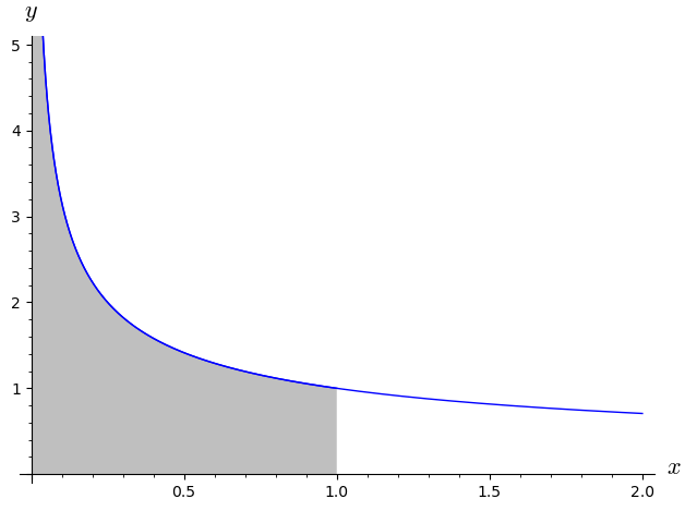
We Must Check Interior Discontinuities!
If an integrand \(f(x)\) has an asymptote at a point \(c\) inside the interval \((a, b)\), we need to split the integral into separate limits: \[ \int_a^b f(x) \mathop{}\!\mathrm{d}x = \int_a^c f(x) \mathop{}\!\mathrm{d}x + \int_c^b f(x) \mathop{}\!\mathrm{d}x. \] If either piece diverges, the entire integral diverges! Ignoring an interior asymptote and applying the Fundamental Theorem of Calculus can lead to nonsensical answers.
Let us see what happens when we compare two functions across an interior asymptote at \(x = 0\).
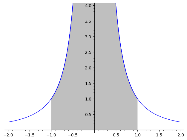
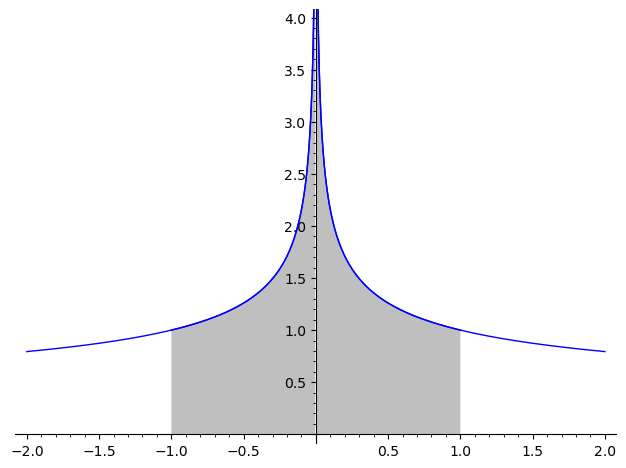
Example 6.3 (Evaluating \(\int_{-1}^1 \frac{1}{x^2} \mathop{}\!\mathrm{d}x\)) The function \(\frac{1}{x^2}\) has a vertical asymptote at \(x = 0\). If we integrate across this discontinuity without checking for asymptotes, we (erroneously) compute: \[ \left[ -\frac{1}{x} \right]_{-1}^1 = (-1) - (1) = -2 \quad \text{ (FALSE!)} \] Something has gone wrong—the graph of \(\frac{1}{x^2}\) lies entirely above the \(x\)-axis, so its area cannot be negative! Instead, properly splitting the integral at \(x = 0\), we must consider: \[ \int_{-1}^1 \frac{1}{x^2} \mathop{}\!\mathrm{d}x = \lim_{t \to 0^-} \int_{-1}^t \frac{1}{x^2} \mathop{}\!\mathrm{d}x + \lim_{s \to 0^+} \int_s^1 \frac{1}{x^2} \mathop{}\!\mathrm{d}x. \] Evaluating just the right-hand piece gives \[ \lim_{s \to 0^+} \int_s^1 \frac{1}{x^2} \mathop{}\!\mathrm{d}x = \lim_{s \to 0^+} \left[ -\frac{1}{x} \right]_s^1 = \lim_{s \to 0^+} \left( -1 + \frac{1}{s} \right) = \infty. \] Since this piece diverges to \(\infty\), the entire integral diverges.
Example 6.4 (\(\int_{-1}^1 \frac{1}{\sqrt[3]{x}} \mathop{}\!\mathrm{d}x\)) Here \(f(x) = x^{-1/3}\) also has an asymptote at \(x = 0\). Splitting at \(x = 0\) gives: \[ \int_{-1}^1 x^{-1/3} \mathop{}\!\mathrm{d}x = \lim_{t \to 0^-} \int_{-1}^t x^{-1/3} \mathop{}\!\mathrm{d}x + \lim_{s \to 0^+} \int_s^1 x^{-1/3} \mathop{}\!\mathrm{d}x. \] Evaluating each limit separately: \[ \lim_{t \to 0^-} \left[ \frac{3}{2} x^{2/3} \right]_{-1}^t = \frac{3}{2}(0) - \frac{3}{2}(1) = -\frac{3}{2}, \] \[ \lim_{s \to 0^+} \left[ \frac{3}{2} x^{2/3} \right]_s^1 = \frac{3}{2}(1) - \frac{3}{2}(0) = \frac{3}{2}. \] Both limits exist, so the integral converges to \(-\frac{3}{2} + \frac{3}{2} = 0\).
Comparing the graphs gives intuition as to why \(\int_0^1 \frac{1}{x^2} \mathop{}\!\mathrm{d}x\) diverges while \(\int_0^1 \frac{1}{\sqrt[3]{x}} \mathop{}\!\mathrm{d}x\) converges:
Often, we only need to know whether an improper integral converges or diverges, rather than finding its exact value (which may be impossible analytically). In such cases, we compare our integrand to a simpler, known benchmark function.
Direct Comparison Test (Stewart et al. 2020, 7.8, pp. 548)
Suppose \(f\) and \(g\) are continuous functions on \([a, \infty)\) satisfying \(0 \le g(x) \le f(x)\) for all \(x \ge a\).
The most difficult part of using this test is knowing which functions to compare our target functions to. In that spirit, we offer an important class of functions whose behavior is well-understood:
Example 6.5 (\(\int_0^{\infty} \frac{1}{x^p} \mathop{}\!\mathrm{d}x\) (Stewart et al. 2020, 7.8, pp. 545–546)) For any \(p > 0\), the graph of \(\frac{1}{x^p}\) tends to 0 as \(x \to \infty\). For which values of \(p\) does the area under the graph converge? We know that when \(p = 1\), the integral becomes \[ \begin{aligned} \int_1^\infty \frac{1}{x} \mathop{}\!\mathrm{d}x & = \lim_{t \to \infty} \int_1^t \frac{1}{x} \mathop{}\!\mathrm{d}x \\ & = \lim_{t \to \infty} \left[ \ln(x) \right]_1^t \\ & = \lim_{t \to \infty} \ln(t) = \infty, \end{aligned} \] and so the integral diverges when \(p = 1\). When \(p \not = 1\), we have \[ \begin{aligned} \int_1^\infty \frac{1}{x^p} \mathop{}\!\mathrm{d}x & = \lim_{t \to \infty} \int_1^t x^{-p} \mathop{}\!\mathrm{d}x \\ & = \lim_{t \to \infty} \left[ \frac{1}{1-p} x^{1-p} \right]_1^t \\ & = \lim_{t \to \infty} \frac{1}{1-p} (t^{1-p} - 1). \\ \end{aligned} \] If the exponent \(1-p\) is greater than \(1\) (i.e., if \(p < 1\)) then this integral runs off to infinity. On the other hand, if \(1-p\) is less than \(1\) (if \(p > 1\)), then the integral converges to the finite number \(\frac{1}{1-p}\). All told we have shown:
The integral \(\int_1^\infty \frac{1}{x^p} \mathop{}\!\mathrm{d}x\) converges if \(p > 1\); otherwise, the integral diverges.
Example 6.6 (\(\int_0^\infty e^{-x^2} \mathop{}\!\mathrm{d}x\)) We split the integral into two parts: \(\int_0^1 e^{-x^2} \mathop{}\!\mathrm{d}x + \int_1^\infty e^{-x^2} \mathop{}\!\mathrm{d}x\). The first integral is finite because \(e^{-x^2}\) is continuous on this interval—since it converges, there is no need to study it further!
For \(x \ge 1\), we have \(x^2 \ge x\), so \(-x^2 \le -x\) and thus \(e^{-x^2} \le e^{-x}\). Evaluating the larger benchmark function gives: \[ \int_1^\infty e^{-x} \mathop{}\!\mathrm{d}x = \lim_{t \to \infty} \left[ -e^{-x} \right]_1^t = \lim_{t \to \infty} \left( -e^{-t} + e^{-1} \right) = \frac{1}{e}. \] Since \(\int_1^\infty e^{-x} \mathop{}\!\mathrm{d}x\) converges, by the Direct Comparison Test, \(\displaystyle \int_0^\infty e^{-x^2} \mathop{}\!\mathrm{d}x\) converges.
f_plot = plot(e^(-x), (x, 0, 4), color='blue', legend_label='$f(x)$')
f_shade = plot(e^(-x), (x, 1, 4), color='blue', fill=True, fillcolor='powderblue', fillalpha=0.5)
g_plot = plot(e^(-x^2), (x, 0, 4), color='red', legend_label='$g(x)$')

show(f_plot + f_shade + g_plot)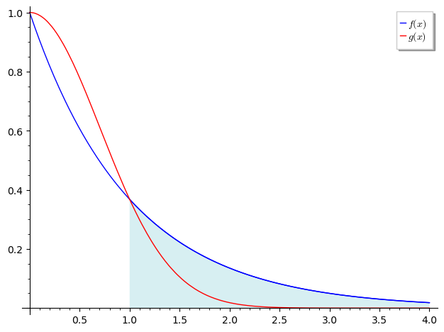
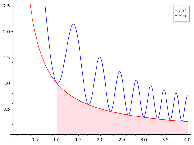
Example 6.7 (\(\int_1^\infty \frac{2+\cos(\pi x^2)}{x} \mathop{}\!\mathrm{d}x\)) For all \(x \ge 1\), we have \(\cos(\pi x^2) \geq -1\) and so \(1 + \cos(\pi x^2) \geq 0\). Therefore: \[ 0 < \frac{1}{x} < \frac{2+\cos(\pi x^2)}{x} \quad \text{for all } x \ge 1. \] We test our smaller benchmark function (or refer to Example 6.5 with \(p=1\)): \[ \int_1^\infty \frac{1}{x} \mathop{}\!\mathrm{d}x = \lim_{t \to \infty} \Big[ \ln\vert{}x\vert{} \Big]_1^t = \lim_{t \to \infty} \ln(t) = \infty. \] Since the smaller integral diverges, \(\displaystyle \int_1^\infty \frac{2+\cos(\pi x^2)}{x} \mathop{}\!\mathrm{d}x\) also diverges.
f_plot = plot((2+cos(pi*x^2))/x, (x, 0, 4), color='blue', legend_label='$f(x)$')
g_plot = plot(1/x, (x, 0, 4), color='red', legend_label='$g(x)$')
g_shade = plot(1/x, (x, 1, 4), color='red', fill=True, fillcolor='pink', fillalpha=0.5)

show(f_plot + g_plot + g_shade, ymax=2.5)