var('x y z')
plane = implicit_plot3d(
y == x,
(x, -2, 2), (y, -2, 2), (z, -2, 2),
)
cylinder = implicit_plot3d(
x^2 + y^2 == 1,
(x, -2, 2), (y, -2, 2), (z, -2, 2),
color = 'red', opacity = 0.5
)
show(plane + cylinder)10 Three-Dimensional Space and Vectors
SageMath Spotlight
- Plotting 3D Surfaces (Section 2.4)
plot_3d(f, (x, xmin, xmax), (y, ymin, ymax))implicit_plot3d(f, (x, xmin, xmax), (y, ymin, ymax), (z, zmin, zmax))- Important options:
color='red'andopacity=0.5
- Defining and Plotting Vectors:
v = vector([1, 2, 3])w = vector([4, 5, 6])- Basic algebra:
v + w,3 * v - Plotting:
arrow3d((0,0,0), v, color='red')
10.1 Three-Dimensional Coordinate Systems
To build more sophisticated models of our physical world, we need to move beyond the \(xy\)-plane into higher-dimensional space: we start with the three-dimensional spatial world, denoted \(\mathbb{R}^3\), where we can rely on a mix of physical intuition and low-dimensional miracles. To do this, we will introduce a third axis, the \(z\)-axis, perpendicular to both the \(x\)- and \(y\)-axes. Note, however, that there are two ways that we could do so! To ensure we all agree on directions, we orient using the Right-Hand Rule:
The Right Hand Rule (Stewart et al. 2020, 12.1, pp. 830)
Here are two equivalent versions of the rule, both of which rely on the use of our right hand (the left hand will give the exact wrong answer). We can pick the one that works best for us!
- Pointing our fingers in the direction of the positive \(x\)-axis and curling them toward the positive \(y\)-axis, our thumb points along the positive \(z\)-axis.
- Pointing our index finger straight along the positive \(x\)-axis and our middle finger perpendicular to it along the positive \(y\)-axis, our thumb, again, points in the positive \(z\)-direction.
Every point in space is now represented by an ordered triple: \((x, y, z)\). Just as the \(x\)- and \(y\)-axes divide the plane into four quadrants, the \(xy\)-, \(yz\)-, and \(xz\)-coordinate planes divide 3D space into eight octants. We can project any point \((x,y,z)\) onto these planes by dropping the irrelevant coordinate (e.g., its projection onto the \(xy\)-plane is \((x, y, 0)\)) (Stewart et al. 2020, 12.1, pp. 831).
Surfaces and Curves
In \(\mathbb{R}^2\), a single equation like \(y = x\) or \(x^2 + y^2 = 1\) describes a 1-dimensional curve (a line and a circle, respectively). What do these equations describe in \(\mathbb{R}^3\)?
Because \(z\) is absent from the equation, \(z\) can be anything without changing the truth value of \(x^2+y^2=1\). Indeed, the circle \(x^2 + y^2 = 1\) is drawn in the \(xy\)-plane, and then stretched infinitely up and down the \(z\)-axis. The result is a 2-dimensional surface—specifically, a cylinder!
Rule of Thumb
Given a system of equations in some number of variables, we expect each equation to drop the dimension of the resulting geometric object by \(1\).
- In the plane, one equation cuts out a curve.
- In 3D space, one equation cuts out a surface.
- To isolate a curve, we need the intersection of two equations.
For example, the circle in the \(xy\)-plane requires two equations: \(x^2 + y^2 = 1\) and \(z = 0\).
Distance and Spheres
The familiar distance formula in \(\mathbb{R}^2\) extends naturally to \(\mathbb{R}^3\) via a double application of the Pythagorean theorem. The distance between points \(P(x_1, y_1, z_1)\) and \(Q(x_2, y_2, z_2)\) is: \[ \vert{}PQ\vert{} = \sqrt{(x_2-x_1)^2 + (y_2-y_1)^2 + (z_2-z_1)^2}. \]
By definition, a sphere is the set of all points \((x,y,z)\) that lie at a constant distance \(r\) (the radius) from a fixed center point \((h,k,l)\). Squaring both sides of the distance formula gives the standard equation of a sphere (Stewart et al. 2020, 12.1, pp. 833): \[ (x-h)^2 + (y-k)^2 + (z-l)^2 = r^2. \]
A Gallery of Quadric Surfaces
Just as conic sections (ellipses, parabolas, hyperbolas) are curves defined by degree-two equations in \(\mathbb{R}^2\), quadric surfaces (Stewart et al. 2020, 12.6, pp. 876) are the 3D surfaces defined by degree-two equations in three variables. These are the most important examples to recognize:
- Spheres and Ellipsoids: If we distort a sphere \(x^2 + y^2 + z^2 = r^2\) by scaling the axes differently, we get an ellipsoid: \[ \frac{x^2}{a^2} + \frac{y^2}{b^2} + \frac{z^2}{c^2} = 1, \] where \(a\), \(b\), and \(c\) are the principal semi-axes.
- Hyperbolic Paraboloid (aka the Saddle): The surface \(z = x^2 - y^2\) curls upward in the \(x\)-direction and downward in the \(y\)-direction. This will be a very important example in our units on optimization!
- Paraboloids and Cones: The paraboloid (\(z = x^2 + y^2\)) is the standard bowl shape. The cone (\(z^2 = x^2 + y^2\)) grows linearly outward from the origin rather than quadratically.
- Cylinders: As we saw earlier, equations missing a variable form cylinders. We can have elliptic cylinders (\(x^2+y^2=1\) or \(x^2 + \frac{y^2}{4} = 1\)) and hyperbolic cylinders (\(x^2 - y^2 = 1\)).
- Hyperboloids: These come in a one-sheeted (\(x^2 + y^2 - z^2 = 1\)) and two-sheeted variety (\(x^2 + y^2 - z^2 = -1\)).
var('x y z')
ellipsoid = implicit_plot3d(x^2/2^2 + y^2/3^2 + z^2 == 1, (x,-3,3), (y,-3,3), (z,-3,3), color='blue')
saddle = plot3d(x^2 - y^2, (x,-2,2), (y,-2,2), color='red', opacity=0.8)
cone = implicit_plot3d(z^2 == x^2 + y^2, (x,-2,2), (y,-2,2), (z,-2,2), color='green', opacity=0.8)
paraboloid = implicit_plot3d(z == x^2 + y^2, (x,-2,2), (y,-2,2), (z,-2,2), color='purple')
elliptical_cylinder = implicit_plot3d(x^2 + y^2 == 1, (x,-2,2), (y,-2,2), (z,-2,2), color='aqua')
hyperbolic_cylinder = implicit_plot3d(x^2 - y^2 == 1, (x,-2,2), (y,-2,2), (z,-2,2), color='yellow', opacity=0.8)
one_sheet_hyperboloid = implicit_plot3d(x^2 + y^2 - z^2 == 1, (x,-2,2), (y,-2,2), (z,-2,2), color='orange', opacity=0.5)
two_sheet_hyperboloid = implicit_plot3d(x^2 + y^2 - z^2 == -1, (x,-2,2), (y,-2,2), (z,-2,2), color='magenta')
show(ellipsoid)
show(saddle)
show(cone + paraboloid)
show(elliptical_cylinder + hyperbolic_cylinder)
show(one_sheet_hyperboloid + two_sheet_hyperboloid)Note that these are only ideal models: they can be rotated and distorted as we please!
It’s easiest to tell what kind of quadric surface we are dealing with by comparing what terms appear in it (linear versus quadratic) and their signature (how the terms are being added or subtracted). For example \(3y = 2x^2+z^2\) also defines a paraboloid (bowl), except it opens in the \(y\) direction! See (Stewart et al. 2020, 12.6, 879) for more on this—we will also discuss methods of plotting in Chapter 14.
10.2 Vectors
Mathematical objects are often most fruitfully defined by how they behave. Our working definition of vector will be as a quantity that possesses both a magnitude (length) and a direction, meaning its fundamental operations allow it to be added to other vectors and scaled by numbers, but these latter processes of addition and scaling actually make for a better definition.
Indeed, many real-world quantities behave this way! When two physical forces push on an object, their combined effect is a vector addition; when the wind blows at 20 mph to the northeast, that is a vector. Conversely, quantities that only have magnitude—like temperature, mass, or time—are called scalars.
Geometric Description
Geometrically, we represent a vector as an arrow pointing from an initial point to a terminal point. If \(A\) and \(B\) are points, we write \[ \vec{v} = \overrightarrow{AB} \] for the vector between them. Note that the data of a vector consists of this length and direction, not where it starts: If we draw two arrows with the exact same length pointing in the exact same direction, they are the exact same vector, even if they are drawn in different places on the page.
Vector addition
Because of how they represent displacement, vectors add head-to-tail (Stewart et al. 2020, 12.2, pp. 837). If the vector \(\vec{v}\) moves us from the point \(A\) to the point \(B\), and the vector \(\vec{w}\) moves us from \(B\) to \(C\), then their sum \(\vec{v} + \vec{w}\) is the net displacement directly from \(A\) to \(C\): \[ \overrightarrow{AB} + \overrightarrow{BC} = \overrightarrow{AC}. \]
Vector scaling
Multiplying a vector \(\vec{v}\) by a scalar \(c\) stretches or shrinks its length by a factor of \(\vert{}c\vert{}\). Moreover, if \(c\) is negative, the vector reverses direction!
We can visualize these geometric definitions in SageMath:
u = vector([3, 1])
v = vector([1, 3])
# Vector addition plot
add_plot = arrow2d((0,0), u, color='blue', legend_label='$\\vec{u}$')
add_plot += arrow2d(u, u+v, color='red', legend_label='$\\vec{v}$')
add_plot += arrow2d((0,0), u+v, color='purple', legend_label='$\\vec{u} + \\vec{v}$', width=3)
# Vector scaling plot
scale_plot = arrow2d((0,0), u, color='blue', legend_label='$\\vec{u}$')
scale_plot += arrow2d((0,0.5), vector((0,0.5)) + 2*u, color='green', legend_label='$2\\vec{u}$')
scale_plot += arrow2d((0,1), vector((0,1)) - 0.5*u, color='orange', legend_label='$-0.5\\vec{u}$')
# Note how we base the vectors at different places to show them side by side!
# Show the two graphics at once
graphics_array([add_plot, scale_plot]).show(axes=False, figsize=[8, 4])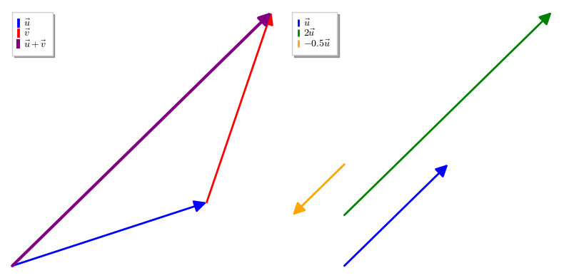
Component Description
To do computation, we need an algebraic representation of these objects. We write a vector in \(\mathbb{R}^3\) using its components in the \(x, y,\) and \(z\) directions, enclosed in angle brackets: \[ \vec{v} = \langle v_1, v_2, v_3 \rangle. \] If we know a vector represents the displacement from a point \(A = (x_1, y_1, z_1)\) to a point \(B = (x_2, y_2, z_2)\), we compute its components by subtracting the initial coordinates from the terminal coordinates (Stewart et al. 2020, 12.2, pp. 839): \[ \overrightarrow{AB} = \langle x_2 - x_1, y_2 - y_1, z_2 - z_1 \rangle. \] By the distance formula, the magnitude (or length) of a vector \(\vec{v} = \langle v_1, v_2, v_3 \rangle\) is the distance from the origin to the point \((v_1, v_2, v_3)\): \[ \left\lVert \vec{v} \right\rVert = \sqrt{v_1^2 + v_2^2 + v_3^2}. \] Any vector with a magnitude of exactly \(1\) is called a unit vector. We can always shrink or stretch a non-zero vector \(\vec{v}\) into a unit vector pointing in the exact same direction by dividing by its own length. We denote unit vectors with a “hat”: \[ \hat{v} \coloneqq \frac{1}{\left\lVert \vec{v} \right\rVert} \vec{v}. \]
Standard Basis Vectors
Three unit vectors are so important that we give them special names. These are the standard basis vectors in \(\mathbb{R}^3\), which point along the positive \(x, y,\) and \(z\) axes: \[ \mathbf{i}= \langle 1, 0, 0 \rangle, \quad \mathbf{j}= \langle 0, 1, 0 \rangle, \quad \mathbf{k}= \langle 0, 0, 1 \rangle. \]
Any vector \(\vec{v} = \langle v_1, v_2, v_3 \rangle\) can be written as a linear combination of these basis vectors: \[ \vec{v} = v_1 \mathbf{i}+ v_2 \mathbf{j}+ v_3 \mathbf{k}. \]
Vectors Act Like Vectors
Because vectors are defined by component-wise arithmetic, they inherit many of the familiar algebraic laws of real numbers (Stewart et al. 2020, 12.2, pp. 840). For any vectors \(\vec{u}, \vec{v}, \vec{w}\) and scalars \(c, d\), we have:
- Commutativity: \(\vec{u} + \vec{v} = \vec{v} + \vec{u}\)
- Associativity: \((\vec{u} + \vec{v}) + \vec{w} = \vec{u} + (\vec{v} + \vec{w})\)
- Additive Identity: \(\vec{u} + \vec{0} = \vec{u}\) (where \(\vec{0} = \langle 0,0,0 \rangle\))
- Additive Inverse: \(\vec{u} + (-\vec{u}) = \vec{0}\)
- Distribution of Scalar over Vector Addition: \(c(\vec{u} + \vec{v}) = c\vec{u} + c\vec{v}\)
- Distribution of Vector over Scalar Addition: \((c + d)\vec{u} = c\vec{u} + d\vec{u}\)
- Compatibility of Scalars: \((cd)\vec{u} = c(d\vec{u})\)
- Scalar Identity: \(1\vec{u} = \vec{u}\)
Whenever we encounter a mathematical object that obeys these exact eight rules, it is fundamentally acting like a vector, even if it doesn’t look like an arrow!
All that we have discussed above makes sense for higher-dimensional spaces—and vectors (often in thousand-dimensional spaces, or bigger!) are used across math and science! Indeed, we can describe a vector in the \(n\)-dimensional space \(\mathbb{R}^n\) using similar notation: \[ \vec{v} \coloneqq \langle v_1, v_2, \dots, v_n \rangle. \]