22 Double Integrals I

22.1 Introduction

Big idea

If \(f(x,y)\) is a function defined over a planar region \(R\), we can write \[ \iint_R f(x,y) \mathop{}\!\mathrm{d}A \] for the volume of the solid under the graph of \(f\) and above \(R\): the double integral of \(f(x,y)\) over \(R\).

To define such a quantity, we need to partition \(R\) into small rectangles, then consider the limit of Riemann sums as the partition becomes finer—see (Stewart et al. 2020, figs. 15.1.4–5).

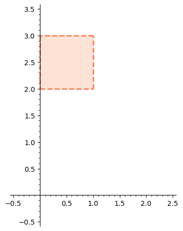
Example: Volume under \(f(x,y) = x^2 y\) over the region \([0,1] \times [2,3]\).

As with a single variable, integrals have some nice properties that help us compute them. In particular:

Linearity

If \(f(x,y)\) and \(g(x,y)\) are continuous on a region \(R\) and \(a\) and \(b\) are constants, then \[ \iint_R \left( a f(x,y) + b g(x,y) \right) \mathop{}\!\mathrm{d}A = a \iint_R f(x,y)\ \mathop{}\!\mathrm{d}A + b \iint_R g(x,y) \mathop{}\!\mathrm{d}A. \]

22.2 Main results

Fubini’s theorem (Stewart et al. 2020, 15.1.10)

If \(f(x,y)\) is continuous on a rectangular region \(R = [a,b] \times [c,d]\), then \[ \iint_R f(x,y) \mathop{}\!\mathrm{d}A = \int_a^b \left( \int_c^d f(x,y) \mathop{}\!\mathrm{d}y \right) \mathop{}\!\mathrm{d}x = \int_c^d \left( \int_a^b f(x,y) \mathop{}\!\mathrm{d}x \right) \mathop{}\!\mathrm{d}y. \]

Example: Area under \(f(x,y) = x^2 y\) over the region \([0,1] \times [2,3]\).

By Fubini’s theorem, we can compute this integral in two ways:

\[ \begin{split} \iint_R x^2 y \mathop{}\!\mathrm{d}A & = \int_0^1 \int_2^3 x^2 y \mathop{}\!\mathrm{d}y \mathop{}\!\mathrm{d}x = \int_0^1 \tfrac{5}{2} x^2 \mathop{}\!\mathrm{d}x = \tfrac{5}{6} \\ & = \int_2^3 \int_0^1 x^2 y \mathop{}\!\mathrm{d}x \mathop{}\!\mathrm{d}y = \int_2^3 \tfrac{1}{3} y \mathop{}\!\mathrm{d}y = \tfrac{5}{6}. \end{split} \]

The first of these—where we hold \(x\) constant, integrate along \(y\), and then add up these slices in \(x\)—is shown in the first figure below; the second is the last figure.

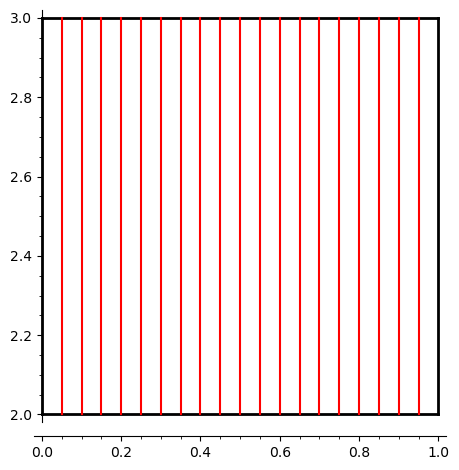
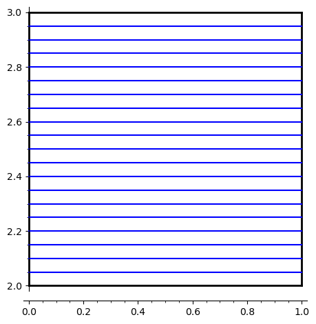
We emphasize that the integrands in the penultimate step of each calculation above—\(\frac{5}{2} x^2\) and \(\frac{1}{3} y\), respectively—represent the area of each slice being integrated to compute the final volume, as shown below:

Each slice has area \(\frac{5}{2} x^2\).

Each slice has area \(\frac{1}{3} y\).

SageMath

You should practice these integrals by hand!—but you should also use Sage to check your work. We can compute \(\int_0^1 \int_2^3 x^2 y \mathop{}\!\mathrm{d}y \mathop{}\!\mathrm{d}x\) via the following:

Listing 22.1: Holding \(x\) constant first

(x^2*y).integrate(y, 2, 3).integrate(x, 0, 1)

5/6

Similarly, \(\int_2^3 \int_0^1 x^2 y \mathop{}\!\mathrm{d}x \mathop{}\!\mathrm{d}y\) is computed here:

Listing 22.2: Holding \(y\) constant first

(x^2*y).integrate(x, 0, 1).integrate(y, 2, 3)

5/6

Double integrals of separable functions (Stewart et al. 2020, 15.1.11)

If we can factor \(f(x,y) = g(x)h(y)\), then we have: \[ \iint_R g(x)h(y) \mathop{}\!\mathrm{d}A = \left( \int_a^b g(x) \mathop{}\!\mathrm{d}x \right) \left( \int_c^d h(y) \mathop{}\!\mathrm{d}y \right). \]

22.3 More interesting regions

Example: Area under \(f(x,y) = x + y\) bound by \(y = 0, x = 1\), and \(y = x^2\).

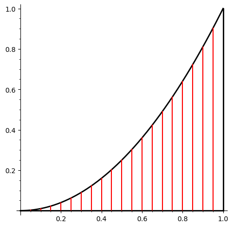
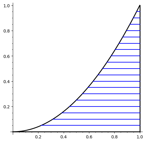
We check both ways of computing the integral:

\[ \begin{split} \iint_R (x+y) \mathop{}\!\mathrm{d}A & = \int_0^1 \int_0^{x^2} (x+y) \mathop{}\!\mathrm{d}y \mathop{}\!\mathrm{d}x = \int_0^1 (\tfrac{1}{2} x^4 + x^3) \mathop{}\!\mathrm{d}x = \tfrac{7}{20} \\ & = \int_0^1 \int_{\sqrt{y}}^1 (x+y) \mathop{}\!\mathrm{d}x \mathop{}\!\mathrm{d}y = \int_0^1 (-y^{3/2} + \tfrac{1}{2}y + \tfrac{1}{2} ) \mathop{}\!\mathrm{d}y = \tfrac{7}{20}. \end{split} \]

Is it easier to hold \(x\) constant first or \(y\) constant first?

Example: Area under \(f(x,y) = x^2 + y^2 + 1\) bound by \(y = 1, y = x, x = -1\), and \(x = 0\).

The volume of interest is shown here:

Our methods for slicing up the region of integration are either of the following:

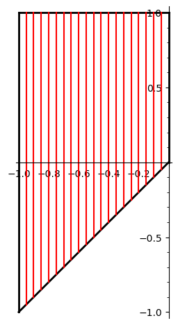
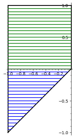
The volume is \(\frac{5}{2}\). Is it easier to hold \(x\) constant first or \(y\) constant first?

SageMath

We can use Sage to compute integrals over non-rectangular regions as well!

We compute \(\int_0^1 \int_0^{x^2} (x+y) \mathop{}\!\mathrm{d}y \mathop{}\!\mathrm{d}x\):

integrate(
    integrate(
        x + y,
        (y, 0, x^2)
    ),
    (x, 0, 1)
)

7/20

We compute \(\int_{-1}^0 \int_x^1 (x^2+y^2+1) \mathop{}\!\mathrm{d}y \mathop{}\!\mathrm{d}x\):

integrate(
    integrate(
        x^2 + y^2 + 1,
        (y, x, 1)
    ),
    (x, -1, 0)
)

5/2

Warning

The inner variable should not appear in the outer integral limits—you know something has gone wrong in your setup if that happens!

22.4 Homework

(Stewart et al. 2020, sec. 15.1) #6, 15–18
(Stewart et al. 2020, sec. 15.2) #1–4