a = 6 # Take the number 6, put it in a box named 'a'
b = 3 # Take the number 3, put it in a box named 'b'
# Add the content of the boxes together
# This is the last line of the cell, so the result is automatically printed
a + b9This page is a reference. As such, it is not meant to be read cover-to-cover in one sitting, but rather to be skimmed for big ideas, then intentionally consulted! The goal here is to help someone with little to no experience in coding get a start in translating mathematical ideas into a language that our computers can understand. We will refer to this page regularly throughout the course, especially when working on Homework and Group Quizzes.
We’ll be using SageMath (more commonly referred to by its older name, Sage1), which is free, open-source math software trusted by researchers and hobbyists alike. Because Sage is built on top of Python, we will develop two valuable skill sets at once: Python’s foundational programming concepts (which translate readily to other modern languages) and Sage’s domain-specific mathematical commands.
To actually write and execute SageMath code, we need a way to access it! We will focus on a friendly, visual tool called a Jupyter Notebook to do the heavy lifting, but we will mention three distinct avenues for getting up and running.
When working on mathematics, sometimes we just need to quickly evaluate a single expression or generate a quick plot without opening a full workspace. To do this, we can use a web browser to visit SageMathCell, which is a free, web-based sandbox. We can hammer out a few lines of code, click “Evaluate”, and see the result!
Running SageMath entirely on your own machine means you don’t have to rely on an active internet connection. This is recommended if you plan to continue programming in future math, science, or data analytics courses!
Carleton Setup Guides
If you are installing SageMath on your personal computer, Technical Director Mike Tie has put together step-by-step documentation just for us:
Official installation instructions are posted and maintained by SageMath developers. For those using macOS or Linux, an efficient way to get up and running is via a package manager like Homebrew or Conda. For an introduction to these ideas, check out my introductory guide on package managers.
Be careful with terminal commands you find online!
Never paste commands containing curl or sudo into your terminal unless you trust the source. Running unverified shell scripts can modify critical system settings or execute malicious code.
Once a package manager is set up, installing and running SageMath is as easy as running the appropriate commands in your terminal.
macOS (via Homebrew): First we can install Homebrew by launching the Terminal application and executing the command:
/bin/bash -c "$(curl -fsSL https://raw.githubusercontent.com/Homebrew/install/HEAD/install.sh)"After the installation finishes, installing SageMath is easy:
brew install --cask sageWindows (WSL) & Ubuntu (via Miniforge / Conda): Ubuntu ships with the apt (Advanced Package Tool) package manager. Sadly, recent Ubuntu releases no longer carry SageMath in apt, so the installation is more involved. The current recommended route is via Miniforge.
Hit WindowsWindows, type “Ubuntu” to find the entry in the Microsoft Store, and install the app. Launch it, create a username (letters, numbers, and underscores are allowed) and password (there is no feedback as you type—this is a standard security measure), and proceed with any additional setup. Then run the following command:
curl -L -O "https://github.com/conda-forge/miniforge/releases/latest/download/Miniforge3-$(uname)-$(uname -m).sh"
bash Miniforge3-$(uname)-$(uname -m).shPress EnterEnter, then ↓↓ to scroll through the terms, enter “yes” when prompted, and confirm the installation location. Once this is done, initialize the package manager, refresh the terminal, and install SageMath wih this code:
~/miniforge3/bin/conda init
source ~/.bashrc
conda create -n sage -c conda-forge sage -ySageMath is installed at this point! You can launch by running conda activate sage && sage -n jupyter. However, by default, Conda requires you to manually activate environments before using them— you will need to run conda activate sage every time you open a terminal before launching Sage. Let’s fix that!
To make sage and sage -n jupyter work immediately in any fresh terminal session (just like on macOS), add an alias to your shell configuration, then refresh the shell:
echo 'sage() { conda activate sage; command sage "$@"; conda deactivate; }' >> ~/.bashrc
source ~/.bashrcArch Linux (via pacman): Launch your favorite terminal emulator and run:
sudo pacman -S sagemathIf you run into installation hiccups on your personal laptop, or if you prefer to avoid the process altogether, you don’t have to worry!
Configured installations of SageMath and the Jupyter Notebook environment are available on the desktop workstations located in the Center for Mathematics and Computing (CMC) labs: check CMC 304 and CMC 307! These labs also serve as an excellent workspace for group projects and homework sessions.
A Jupyter Notebook is an interactive, browser-based environment that lets us mix formatted instructions, live code, and math visualizations in a single document. Such notebooks are broken down into small, manageable chunks called cells, which we can run one at a time and in any order we like.
We can write a few lines of code in a cell, execute it (usually by pressing ), and the results—like a 3D plot or a solved algebraic equation—will appear beneath it. This step-by-step process is very forgiving and fantastic for visual exploration.
When we start SageMath, it spins up a local web server on your computer and automatically opens a new tab in your default web browser. Even though it’s running in Chrome, Safari, Firefox, etc., this process is local to your machine and doesn’t require an internet connection!
sage -n jupyterOn Windows, you’ll see a flurry of information including a URL (typically beginning with http://localhost:8888/). You can hold CtrlCtrl and click to open in your favorite browser!
Once the browser dashboard opens, navigate to the folder where you want to work, click the New button in the top right corner, and select SageMath from the dropdown menu to create a blank notebook.
A great way to learn about these notebooks is to experiment with them!
Programming can feel pedantic—computers do what we type, which is often not what we mean! Before writing actual code, we’ll start with comments, which are notes embedded in our programs to provide context for other programmers. Writing clear comments is a core part of documenting our code, ensuring that others (and our future selves!) can easily understand the purpose and logic of what we’ve written.
In mathematical notation, an equals sign usually reflects some notion of balance—when we use it in an equation, we mean that the value, amount, or expression on the left is exactly equivalent to the one on the right. On the other hand, in Python, a single equals sign = represents a fundamentally asymmetrical action: it takes whatever is on the right side and stores it in a sort of “box” (a variable) named by the left side. This is called assignment.
a = 6 # Take the number 6, put it in a box named 'a'
b = 3 # Take the number 3, put it in a box named 'b'
# Add the content of the boxes together
# This is the last line of the cell, so the result is automatically printed
a + b9Naming Rules: Python variable names must follow a few basic conventions:
snake_case), like my_first_variable.Total and total and TOTAL are all treated as different variables).In mathematics, we often use names like \(x\) and \(y\) for our variables. In computer science, on the other hand, good variable names are descriptive and help us make sense of what the code is actually doing. We will strive for a balance between these conventions in this course!
If a single equals sign assigns a value, how do we write a mathematical equation, or check if two variables are equal? The convention in Python, as in many other programming languages, is to use a double equals sign ==. We should think of == as asking the computer a question: “Are these two things the same?” or as declaring a rigid mathematical truth. Other common comparisons we might use are:
< is the left-hand side smaller than the right-hand side?> is the left-hand side greater than the right-hand side?<= is the left-hand side smaller than or equal to the right-hand side?>= is the left-hand side greater than or equal to the right-hand side?!= is the left-hand not equal to the right-hand side?We can store the result of such a question into a variable, or use it directly as in Section 2.2.9. We demonstrate this below, using the print() function to output the result:
x = 7
equal_to_7 = (x == 7)
print("Is x equal to 7?", equal_to_7)
less_than_6 = (x < 6)
print("Is x less than 6?", less_than_6)Is x equal to 7? True
Is x less than 6? FalseIn computer science, a variable that is equal to True or False is called a boolean.
Given an equation (or inequality), we can recover its left or right-hand side by using the .lhs() and .rhs() methods, respectively:
var('x y')
equation = (x^5+x == -y)
print("My favorite equation is", equation)
print("The left-hand side is", equation.lhs())My favorite equation is x^5 + x == -y
The left-hand side is x^5 + xWhen translating math to code, we must explicitly write out our operations. The computer does not understand implied multiplication! 2x will cause an error; we must write 2*x. For exponents, Sage allows us to use the caret symbol ^ (e.g., x^2).
The caret symbol is often reserved for other operations in programming languages. In Python, for example, one has to write 3**4 to compute \(3^4\).
By default, Sage tries to do math exactly. When we type 1/3, the computer will retain this value as the fraction \(\frac{1}{3}\). Contrast such behavior with your trusty TI-84 or Google’s built-in calculator, both of which would convert the fraction to a decimal expression like \(0.333333\). We can even do nifty calculations like this:
1/2 + 1/35/6Likewise, the square root of 2 is kept as \(\sqrt{2}\)—that is, as some quantity whose square is equal to 2—and pi is kept exactly as \(\pi\).
On the other hand, sometimes we just want an ordinary decimal expansion so we can keep track of what’s what. To force Sage to return such an approximation, we can use the .n() (which stands for numerical approximation) method. 2
exact_result = pi + sqrt(2)
approx_result = exact_result.n()
print("Exact result:", exact_result)
print("Decimal approximation:", approx_result)Exact result: pi + sqrt(2)
Decimal approximation: 4.55580621596289Often, we want to mix text (which must be wrapped in quotation marks—computer scientists call these strings) with variables to produce readable output.
A convenient way to do this is using an f-string (formatted string): we put an f right before the quotation marks, then inject variables directly into the text using curly braces {}.
name = "Euler"
favorite_number = 2.718281828459045
print(f"My name is {name} and I like the number {favorite_number}.")My name is Euler and I like the number 2.71828182845905.Python is a very general-purpose language—this is one of its core strengths, and part of what makes it so ubiquitous across so many fields of study. In particular, Python doesn’t automatically know that x or y are mathematical symbols! If we try to do mathematics with a letter that we haven’t properly introduced to the computer, the software will throw an error. Instead, we should properly declare our symbolic variables using var().
var('x y t')
exp1 = 4*x^2 - y
exp2 = x^2 - t
exp1 - exp23*x^2 + t - yAn expression is just a mathematical phrase stored in a variable. To evaluate an expression at a specific number, we can use the .subs() (substitute) command.
var('x y')
z = x^4 + y^4 - 4*x*y
z_val = z.subs(x=1,y=-1)
print(f"{z} at (x,y)=(1,-1) is equal to {z_val}") x^4 + y^4 - 4*x*y at (x,y)=(1,-1) is equal to 6On the other hand, a callable function is defined with parentheses—we should think of it as functions like \(f(x)\) from mathematics courses. We can “plug” numbers directly into these functions without needing the .subs() command:
var('x')
f(x) = x^2 + 5
f(-3)14A list is a fundamental datatype in computer programming. Fortunately, they are exactly what they sound like: a collection of items, kept in a specific order. In Python, lists are created using square brackets [], and the items are separated by commas. In this class, we might use lists to represent coordinates, collections of equations, or sets of solutions.
some_numbers = [2, 4, 6, 8, 10]
print(f"The first element in our list is {some_numbers[0]}")
print(f"Here's another: {some_numbers[3]}")The first element in our list is 2
Here's another: 8Note that the “indexing” in Python (that is, the number we put into the brackets to access specific elements of our lists) begins at 0! In the example above, 2 is the “0-th” element of some_numbers. This is for a good reason, though we will not delve into why here.
Sometimes we only want the computer to run code if a certain condition is met. To accomplish this, we use if statements:
x = 10
if x > 5:
print(f"{x} is a large number!")
print(f"But {x+1} is even larger.")
else:
print(f"I can count {x} with one hand.")
print("This line of code runs no matter what, since it is not indented.")10 is a large number!
But 11 is even larger.
This line of code runs no matter what, since it is not indented.We should think of these sorts of logical statements as the building blocks of interesting programs.
In Python, the code that belongs inside the if statement must be indented (pushed to the right by pressing Tab or Space). This indentation tells Python what code is grouped together—so different indentation will change the logic of our programs! Other languages might use brackets [] or curly braces {} rather than whitespace to logically group bits of code.
Another family of important control structures in computer programming are the various ways of iterating. A for loop allows us to run the same block of (indented) code for every item in a list:
my_list = [1, 2, 6, 5]
# Read this as: "For every entry of 'my_list', do the following:"
for number in my_list:
square = number^2
print(f"The square of {number} is {square}")The square of 1 is 1
The square of 2 is 4
The square of 6 is 36
The square of 5 is 25Throughout this course, we’ll use loops to extract multiple solutions to algebraic equations, generate visualizations, and apply simple rules repeatedly. Instead of copying and pasting the same commands over and over, loops let us write concise, readable code that scales to more complex problems. This aligns with a core principle in computer science: DRY (Don’t Repeat Yourself)!
SageMath has several robust tools for drawing in two dimensions, most of which follow the same pattern:
color=... or linestyle=....show() to control how the finished graphic is displayed.As we work through examples, notice how these patterns appear repeatedly!
To draw a standard function where \(y\) depends on \(x\) (like \(y = x^2\)), we use the plot() command. We must provide the function and the bounds (minimum and maximum \(x\)-values) for the independent variable.
var('x')
plot(x^2, (x, -3, 3), color='red')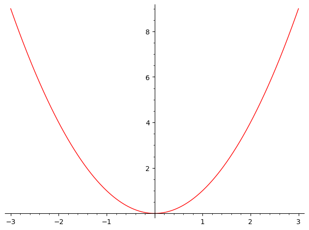
To plot a specific coordinate in the plane, use the point() command. We can pass it a single list [x, y], or a list of lists (shown below) to plot many points at once.
point([[0, 0], [-1, 3], [1, 2], [2, -1]], color='green', size=80)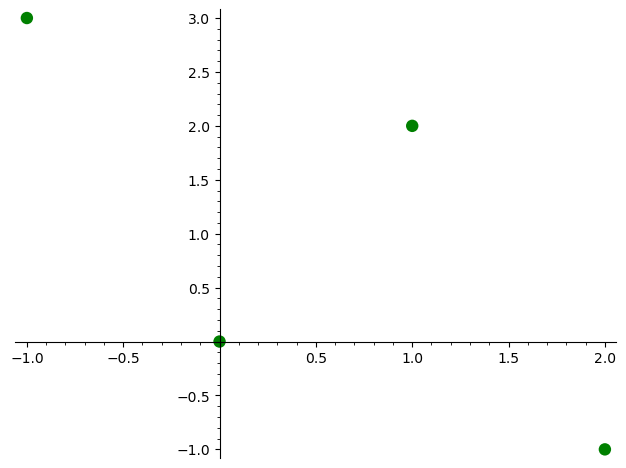
Notice that the plot automatically chooses coordinate ranges large enough to display all the points. The size option controls the size of the plotted markers.
Most Sage plotting commands produce a “graphics object”. If we run multiple plot commands in separate cells, they will draw separate pictures. To overlay them on top of each other, we can save these objects into variables, combine them with the + sign, and display the result using show().
var('x')
curve = plot(sin(x), (x, -pi, 2*pi), color='blue')
dot = point([pi/6, 1/2], color='red', size=60)
show(curve + dot)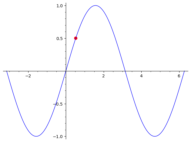
The show() command also accepts options that affect the entire graphic. One particularly useful option is aspect_ratio=1, which ensures that one unit on the x-axis has the exact same visual length as one unit on the y-axis.
Often, an equation cannot be easily rewritten as \(y = f(x)\). For example, the circle of radius \(3\) centered at the origin can be defined as the points \((x,y)\) satisfying \(x^2+y^2=9\). To graph equations where the variables are tangled together in this way, we can use implicit_plot().
var('x y')
implicit_plot(x^2 + y^2 == 9, (x, -4, 4), (y, -4, 4), color='purple')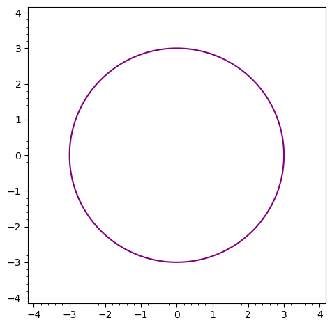
Remember to use the double equals == to define the equation! Furthermore, notice that implicit_plot() requires ranges for both \(x\) and \(y\), since Sage must search a two-dimensional grid for points satisfying the equation.
Our code is getting complicated! While Python usually relies on strict indentation to understand our logic, it makes one very helpful exception: inside parentheses (), brackets [], or braces {}, we can freely break lines wherever we want, since the computer knows the command isn’t finished until it sees the closing symbol. This allows us to break long commands with many arguments into much more readable chunks:
circle = implicit_plot(
x^2 + y^2 == 9,
(x, -4, 4),
(y, -4, 4),
color='purple'
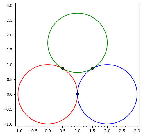
)Remember that we can plot many curves and points at once by using show()!
var('x y')
show(
implicit_plot(x^2 + y^2 == 1, (x,-1,1), (y,-1,1), color='red') +
implicit_plot((x-2)^2 + y^2 == 1, (x,1,3), (y,-1,1), color='blue') +
implicit_plot((x-1)^2 + (y-sqrt(3))^2 == 1, (x,0,2), (y,0,3), color='green') +
point([[1, 0], [1/2, sqrt(3)/2], [3/2, sqrt(3)/2]], color='black', size=50)
)
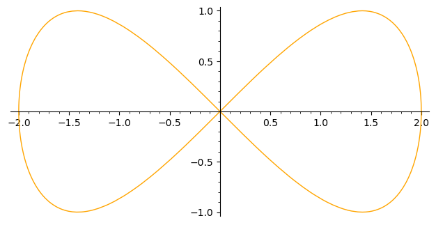
Sometimes, a curve is defined by a separate parameter, often representing some sort of auxiliary property (perhaps \(t\) for time). In such a setup, rather than \(y\) depending on \(x\), both \(x\) and \(y\) depend on \(t\). In order to visualize such a curve, we use parametric_plot() and provide the formulas for \(x(t)\) and \(y(t)\) inside a list, together with the range of parameter values.
var('t')
parametric_plot(
[2*cos(t), sin(2*t)],
(t, 0, 2*pi),
color='orange'
)
A vector field assigns an arrow (a direction and a magnitude) to every point in the plane, often used to describe the “flow” of some varying quantity in a region. We will use plot_vector_field(), which expects a list containing the expressions that describe horizontal flow and vertical flow, respectively.
var('x y')
plt = plot_vector_field(
[-y, x],
(x, -3, 3),
(y, -3, 3),
plot_points=15
)
show(plt, aspect_ratio=1)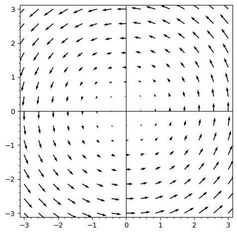
The first expression gives the horizontal component of each vector, while the second gives the vertical component. The plot_points option controls how densely the field is sampled: Larger values produce more arrows and reveal finer detail!
Closely related is the slope field, which visualizes the family of solutions to a first-order differential equation \(\frac{dy}{dx} = f(x,y)\). Instead of plotting directional arrows with varying magnitudes, plot_slope_field() draws uniform line segments representing the slope \(f(x,y)\) at each grid point.
var('x y')
plt_slope = plot_slope_field(
y * (4-y) * sin(x),
(x, 0, 3*pi),
(y, 0, 5.4),
plot_points=20
)
show(plt_slope, aspect_ratio=1)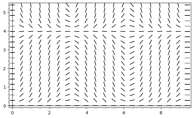
We can decorate these further using numerically computed integral curves: the streamline_plot() function draws trajectories at various initial values.
plt_stream = streamline_plot(
y * (4-y) * sin(x),
(x, 0, 3*pi),
(y, 0, 5.4),
plot_points=20
)
show(plt_slope + plt_stream, aspect_ratio=1)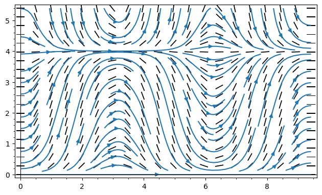
When we add a third variable, things become much harder to visualize on paper. There is where SageMath and other graphing software shines!
If height (\(z\)) is determined directly by a formula involving \(x\) and \(y\), we use plot3d().
var('x y')
plot3d(
x^2 - y^2,
(x, -2, 2),
(y, -2, 2),
color='cyan',
opacity=0.8
)The opacity option (ranging from 0.0 to 1.0) controls transparency. Making a surface slightly transparent is incredibly useful when visualizing multiple surfaces simultaneously or looking at curves hidden underneath! Note that we can click, scroll, and drag the resulting 3D figure to view it from multiple perspectives.
Just as circles are implicit curves in the plane, spheres are implicit surfaces in space.
var('x y z')
implicit_plot3d(
x^2*y^2 + x^2*z^2 + y^2*z^2 == 1,
(x, -3, 3),
(y, -3, 3),
(z, -3, 3),
color='red'
)Because the surface could exist anywhere in space, we must provide boundaries for \(x\), \(y\), and \(z\). As before, we can combine plots using show():
var('x y z')
plt1 = plot3d(
x^2 - y^2,
(x, -2, 2),
(y, -2, 2),
color='cyan',
opacity=0.8
)
plt2 = implicit_plot3d(
x^2 + y^2 + z^2 == 4,
(x, -2, 2),
(y, -2, 2),
(z, -2, 2),
color='purple'
)
show(plt1 + plt2)A particle moving through space traces out a 3D curve whose coordinates all depend on a single parameter (\(t\)).
var('t')
x_val = cos(t)
y_val = sin(t)
z_val = t / 5
parametric_plot3d(
[x_val, y_val, z_val],
(t, 0, 4*pi),
color='green',
thickness=5
)Instead of looking at a 3D surface from the side, sometimes we want to look at it straight down from above, drawing lines where the elevation is constant (like a topographical map). In mathematics, this is referred to as a contour plot, which displays the level curves of a surface. We use contour_plot():
var('x y')
contour_plot(
x^3 + y^3 - 3*x*y,
(x, -2, 2),
(y, -2, 2),
contours=15,
cmap='viridis'
)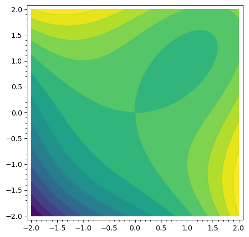
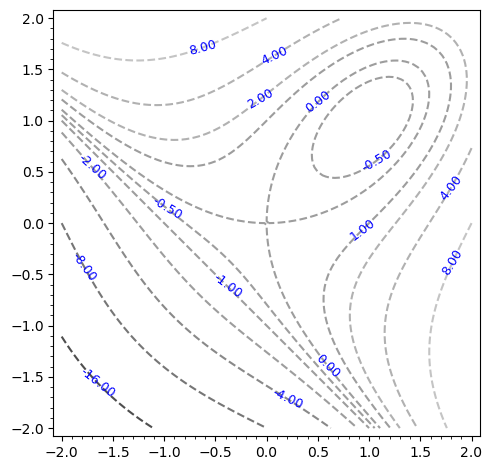
The contours option controls how many level curves are drawn, while cmap selects the color scheme used to represent different heights. We can also make ink-friendly versions of these diagrams using the fill=False command, or apply other decorations like linestyles or labels.
var('x y')
contour_plot(
x^3 + y^3 - 3*x*y,
(x, -2, 2),
(y, -2, 2),
contours=[-32, -16, -8, -4, -2, -1, -0.5, 0, 1, 2, 4, 8, 16],
linestyles='--',
labels=True,
fill=False
)
For many students, the most difficult part of a calculus course is not the calculus, but the difficult accompanying algebra. While we must continue to hone our skills in algebraic manipulations, it is often useful to have the computer handle the heavy lifting to verify our work!
We can use the .expand() and .factor() methods to manipulate cumbersome symbolic expressions:
var('x y')
# Multiply an expression out
expr1 = (x + y)*(x - 3)^2
print(f"{expr1} expands to {expr1.expand()}")
# Factor another expression
expr2 = x^2 - 2*x*y + y^2
print(f"{expr2} factors to {expr2.factor()}")(x + y)*(x - 3)^2 expands to x^3 + x^2*y - 6*x^2 - 6*x*y + 9*x + 9*y
x^2 - 2*x*y + y^2 factors to (x - y)^2A very common trick, especially when setting up integrals, is to take a complex fraction and break it apart into simpler, smaller fractions. The .partial_fraction() method does this for us:
var('x')
fraction = 5 / (x^2 - x - 6)
fraction.partial_fraction(x)-1/(x + 2) + 1/(x - 3)Sometimes a function behaves according to different rules on different intervals. In Sage, we can define piecewise functions using a list of pairs. Each pair contains an interval and the formula that applies there: [(interval, formula), (interval, formula)].
var('x')
# Rule 1: From x=-3 to x=0, f(x) = -2x
# Rule 2: From x=0 to x=2, f(x) = x^2
f = piecewise([
((-3, 0), -2*x),
((0, 2), x^2)
])
plot(f, (x, -3, 2))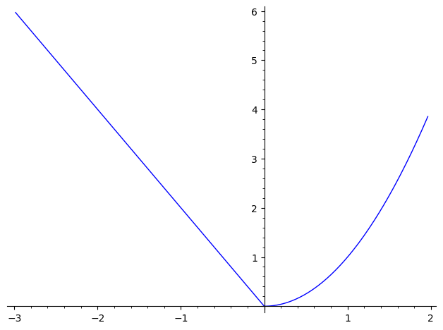
While the piecewise() command is convenient, it simply draws the curves. In particular, it does not automatically generate the traditional open (hollow) and closed (solid) circles we use to denote endpoints and discontinuities!
To get a mathematically precise visual, we can manually plot the functions in their desired ranges and sum them together with show(). Here we produce a plot of the piecewise function \[
f(x) = \left\{ \begin{array}{ll}
\cos x & x < 0 \\
-\frac{1}{2} & x = 0 \\
\frac{x}{x^2+1} & x > 0
\end{array} \right.
\] on the interval \(-4 \leq x \leq 4\). Note that our new approach gives us the control to explicitly draw holes and solid dots using the point() command!
var('x')
left_curve = plot(cos(x), (x, -4, 0))
right_curve = plot(x/(x^2+1), (x, 0, 4))
# Make the "holes" by placing a smaller white dot on top of a darker one!
left_hole = point([0, 1], size=50) + point([0, 1], size=30, color='white')
right_hole = point([0, 0], size=50) + point([0, 0], size=30, color='white')
solid_dot = point([0, -0.5], size=50)
show(left_curve + right_curve + left_hole + right_hole + solid_dot)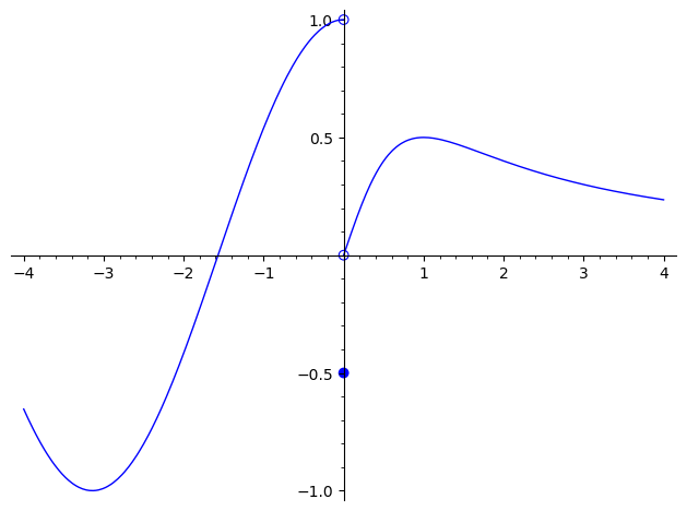
To find exact symbolic solutions to an equation, we use solve(). We must provide this function with the equation (using ==) and the variable that we want to solve for.
var('x')
solve(x^2 - 5*x + 6 == 0, x)[x == 3, x == 2]Notice how the output of solve is a list of equations! We can extract the numbers themselves using the .rhs() method discussed earlier.
var('x')
solutions = solve(x^2 - 5*x + 6 == 0, x)
# Loop through the solutions and print them
print("The solutions are:")
for sol in solutions:
print(sol.rhs())The solutions are:
3
2Often, we need multiple equations (which can involve many variables) to be true at the same time. In such situations, we can pass a list of equations to solve().
Sage tries to be as thorough as possible mathematically, which means it will often return complex numbers (involving the number \(i\), whose square is \(-1\)). For example, the system \[ x^2 y = 1 \quad \text{and} \quad y = x^2 \] has four solutions: \[ (x,y) = (1,1), (-1,1), (i, -1), \text{ and } (-i, -1), \] but only the first two are real. In this course, we are primarily interested in real solutions.
Given a variable containing a number—let’s call it num—we can check whether it is real using num in RR. In order to ignore complex solutions, we use a Python trick called a list comprehension (essentially a for loop squeezed into a single line). We use the all() function, together with the .rhs() method, to check if every value in a given solution is real.
var('x y')
eq1 = x^3 - y == 0
eq2 = y^3 - x == 0
solutions = solve([eq1, eq2], [x, y])
# Filter to only include real solutions
real_solutions = [
sol for sol in solutions
if all(eq.rhs() in RR for eq in sol)
]
print("The real solutions are:")
for sol in real_solutions:
print(sol)The real solutions are:
[x == -1, y == -1]
[x == 1, y == 1]
[x == 0, y == 0]We evaluate limits to see how functions behave near boundaries, holes, or as variables grow without bound. The command is limit().
var('x')
f(x) = sin(x) / x
limit(f(x), x=0)1Sometimes limits differ depending on which direction we approach the target value from. We use the keyword argument dir='+' to approach from the right (larger values sliding down), and dir='-' to approach from the left (smaller values sliding up). Note that we use sqrt(x) below to stand for \(\sqrt{x}\):
var('x')
# Approaching from the right
limit_from_right = limit(sqrt(x), x=0, dir='+')
print(f"Limit of sqrt(x) approaching 0 from the right: {limit_from_right}")
# Approaching from the left
limit_from_left = limit(1/x, x=0, dir='-')
print(f"Limit of 1/x approaching 0 from the left: {limit_from_left}")Limit of sqrt(x) approaching 0 from the right: 0
Limit of 1/x approaching 0 from the left: -InfinityIn Sage, the concept of infinity is represented by two lowercase ’o’s:
limit((6*x^2+1)/(3*x^2-4*x), x=oo)2To compute derivatives in Sage, we use the diff() command (short for differentiate). We must provide the expression, and explicitly tell Sage which variable we are taking the derivative with respect to.
var('x')
f = x^3 + e^(2*x)
print(f"First derivative of {f} is {diff(f, x)}.")
# Add a number at the end to specify how many times to differentiate
print(f"Second derivative is {diff(f, x, 2)}.")First derivative of x^3 + e^(2*x) is 3*x^2 + 2*e^(2*x).
Second derivative is 6*x + 4*e^(2*x).When a relationship between variables is given implicitly (e.g., \(x^2 + y^2 = 25\)), we can still find \(\frac{\mathop{}\!\mathrm{d}y}{\mathop{}\!\mathrm{d}x}\) using Sage’s diff()—but we must treat \(y\) as a function of \(x\) rather than as a standalone variable! In other words, if we want to compute derivatives where one variable is presumed to depend on another, we have to use function('y')(x) to define \(y\) as a function of \(x\).
var('x')
y = function('y')(x)
equation = x^2 + y^2 == 25
print("Original equation:", equation)
diff_equation = diff(equation, x)
print("Differentiated equation:", diff_equation)
# We can even solve for dy/dx
dy_dx = solve(diff_equation, diff(y, x))
# Remember that solve returns a list of solutions; we'll print the first one
print(dy_dx[0])Original equation: x^2 + y(x)^2 == 25
Differentiated equation: 2*y(x)*diff(y(x), x) + 2*x == 0
diff(y(x), x) == -x/y(x)If an expression contains multiple variables (like \(x\), \(y\), and \(z\)), we often need to analyze how the function changes if we change in one specific direction while ignoring the others. Treating one variable as the active variable and all others as fixed constants is called taking a partial derivative. Computationally, the syntax remains exactly the same!
#| lst-label: lst-demo-partial-derivatives
#| lst-cap: Taking derivatives of multi-variable expressions.
var('x y')
f = x^2 * sin(y)
# Differentiate with respect to x (treat y as a constant)
fx = diff(f, x)
# Differentiate with respect to y (treat x as a constant)
fy = diff(f, y)
# Mixed derivative: differentiate with respect to x, then with respect to y
diff(fx, y)Often, we want to collect all of these individual directional rates of change into a single vector (known as the gradient). Rather than computing them one by one, we can get the entire vector at once by calling .gradient() on our function.
var('x y')
f(x, y) = x^2 + 3*y
f.gradient() (x, y) |--> (2*x, 3)While derivatives represent rates of change, integration represents accumulation (like finding the area under a curve, or the volume of a solid). The command is integrate().
If we do not provide geometric bounds, Sage returns the general algebraic formula for the antiderivative (though it assumes we know to add the customary \(+C\) ourselves).
var('x')
f = x * cos(x^2)
integrate(f, x)1/2*sin(x^2)We can achieve the same result using a method, replacing the last line of the above with f.integrate(x).
To find a numerical area or exact accumulated value, we provide the variable, the lower bound, and the upper bound. For example:
var('x')
integrate(x^2, x, 0, 2)8/3reflects the calculation \[ \int_0^2 x^2 \mathop{}\!\mathrm{d}x = \left. \frac{1}{3} x^3 \right|_{x=2} = \frac{8}{3}. \]
Again, we could have used (x^2).integrate(x,0,2) for a method-based approach.
If we are accumulating volume over a 2D or 3D region, we will have to integrate multiple times, working from the inside out. For more on the mathematics, see Chapter 22. In Python, we can chain methods together by stringing dots: f.cmd1().cmd2() and so on.
We should read the following code from left to right: Take the function, integrate it with respect to \(y\), then take that result and integrate it with respect to \(x\).
var('x y')
f = x * y^2
f.integrate(y, 1, 3).integrate(x, 0, 1)13/3The double integral being evaluated is: \[ \begin{aligned} \int_0^1 \left( \int_1^3 x y^2 \mathop{}\!\mathrm{d}y \right) \mathop{}\!\mathrm{d}x & = \int_0^1 \left( \left. \frac{1}{3} x y^3 \right|^{y=3}_{y=1} \right) \mathop{}\!\mathrm{d}x \\ & = \int_0^1 \frac{26}{3} x \mathop{}\!\mathrm{d}x \\ & = \left. \frac{13}{3} x^2 \right|_{x=0}^{x=1} \\ & = \frac{13}{3}. \\ \end{aligned} \]
We can also use a nesting syntax:
var('x y')
integrate(integrate( x * y^2, (y, 1, 3)), (x, 0, 1))13/3Sometimes, an integral is mathematically impossible to solve with a neat, exact formula in terms of the elementary functions we know and love (a classic example is \(\int e^{-x^2} dl{x}\)). If we attempt to run integrate() in these situations, Sage might return the integral without solving it, print out a solution in terms of unfamiliar expressions (like erf(x)), or otherwise fail. On the other hand, if we just need a decimal approximation, we can bypass the exact symbolic engine and use numerical_integral() for a swift result:
var('x')
numerical_integral(e^(-x^2), 0, 1)[0]0.7468241328124271The numerical_integral command behaves slightly differently. This function returns a pair of items: the first is the estimated value of the definite integral in question, and the second is the margin of error (an estimate of how close the estimated answer is from the true answer). We use [0] at the very end of the command here to grab just the 0-th item—the answer!
This comes from the even older name, “SAGE”, which stands for “System for Algebra and Geometry Experimentation.”↩︎
Throughout these notes, we will see many functions, which are different from methods. A method is a function that belongs to an object. Functions are called directly, while methods are called through an object and may access that object’s internal data. You do not need to understand the difference between these in order to succeed in this course!↩︎
Comments
In Python, any text to the right of a hash symbol
#is completely ignored by the interpreter. We use this to leave notes for ourselves and collaborators.