Vector Projection: (v.dot_product(w) / v.dot_product(v)) * v
Thus far, we have only defined how to multiply a vector by a scalar. There are actually several useful ways to define the multiplication of two vectors—one is discussed here, the dot product, and another will be covered in Chapter 12.
11.1 Coordinate Definition and Algebraic Properties
The Dot Product
Given \(\vec{a} = \langle a_1, a_2, a_3 \rangle\) and \(\vec{b} = \langle b_1, b_2, b_3 \rangle\), their dot product is the sum of the products of their corresponding components (Stewart et al. 2020, 12.3, pp. 847): \[
\vec{a} \cdot \vec{b} \coloneqq a_1 b_1 + a_2 b_2 + a_3 b_3.
\]
There is nothing special about doing this operation in \(\mathbb{R}^3\)! Indeed, if we have vectors in \(n\)-dimensional space, we can still describe their dot product by continuing the above formula: \[
\langle a_1,a_2,\dots,a_n \rangle \cdot \langle b_1,b_2,\dots,b_n \rangle \coloneqq a_1 b_1 + a_2 b_2 + \cdots + a_n b_n.
\]
Because it is defined via straightforward arithmetic operations, the dot product satisfies several convenient algebraic properties (Stewart et al. 2020, 12.3, pp. 848):
Relation to Magnitude:\(\vec{a} \cdot \vec{a} = \left\lVert \vec{a} \right\rVert^2\)
In Property 5, notice the distinction between \(\vec{0}\) (the zero vector, which has components) and \(0\) (the scalar number zero). These are different notions of zero! Indeed, also note that the dot product of two vectors is always a scalar!
11.2 Geometric Meaning: Angles and Orthogonality
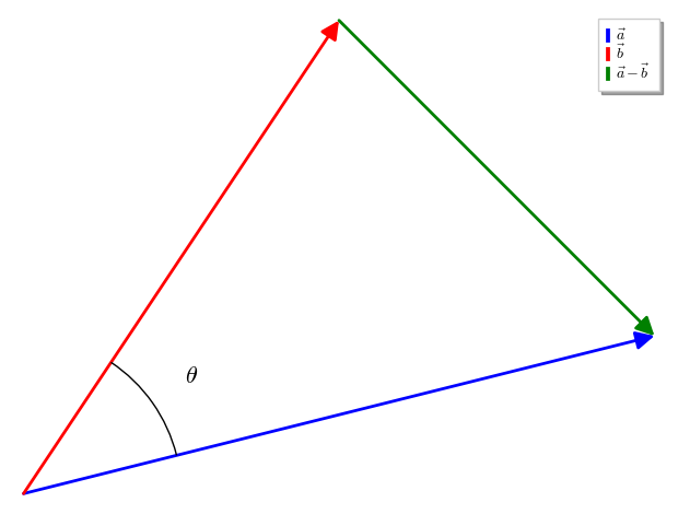
While the coordinate definition is easy to compute, it does not make the geometric power of the dot product immediately apparent. If we place \(\vec{a}\) and \(\vec{b}\) tail-to-tail, the vector connecting their tips is \(\vec{a} - \vec{b}\): This forms a triangle with side lengths \(\left\lVert \vec{a} \right\rVert\), \(\left\lVert \vec{b} \right\rVert\), and \(\left\lVert \vec{a} - \vec{b} \right\rVert\). Consider the following diagram:
The vectors \(\vec{a}\), \(\vec{b}\), and \(\vec{a}-\vec{b}\) form a triangle with angle \(\theta\).
By applying the Law of Cosines to this triangle, \[
\left\lVert \vec{a} - \vec{b} \right\rVert^2 = \left\lVert \vec{a} \right\rVert^2 + \left\lVert \vec{b} \right\rVert^2 - 2\left\lVert \vec{a} \right\rVert\left\lVert \vec{b} \right\rVert\cos\theta,
\] we can deduce the most important theorem of this section (Stewart et al. 2020, 12.3, pp. 848). We expand the left side using the algebraic properties of the dot product: \[
\begin{aligned}
\left\lVert \vec{a} - \vec{b} \right\rVert^2 &= (\vec{a} - \vec{b}) \cdot (\vec{a} - \vec{b}) \\
&= \vec{a} \cdot \vec{a} - \vec{a} \cdot \vec{b} - \vec{b} \cdot \vec{a} + \vec{b} \cdot \vec{b} \\
&= \left\lVert \vec{a} \right\rVert^2 - 2(\vec{a} \cdot \vec{b}) + \left\lVert \vec{b} \right\rVert^2.
\end{aligned}
\] Canceling \(\left\lVert \vec{a} \right\rVert^2\) and \(\left\lVert \vec{b} \right\rVert^2\) yields our geometric formula:
The Dot Product Cosine Formula
If \(\theta\) is the angle between the vectors \(\vec{a}\) and \(\vec{b}\) (with \(0 \le \theta \le \pi\)), then: \[
\vec{a} \cdot \vec{b} = \left\lVert \vec{a} \right\rVert \left\lVert \vec{b} \right\rVert \cos \theta.
\]
This formula relates the algebra of the dot product to the geometry of the underlying vectors! Indeed, we can rewrite it to find the angle between two vectors:
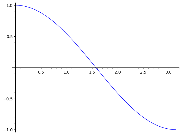
Even better, consider the basic properties of \(\cos \theta\) as \(\theta\) varies between \(0\) and \(\pi\):
var('θ')plot(cos(θ), (θ,0,pi))
In particular, we have \[
\cos \theta \text{ is } \left\{ \begin{array}{ll}
> 0 & \text{if } 0 < \theta < \frac{\pi}{2} \\
= 0 & \text{if } \theta = \frac{\pi}{2} \\
< 0 & \text{if } \frac{\pi}{2} < \theta < \pi. \\
\end{array} \right.
\] Hence we can determine whether two vectors are pointing generally in the same direction (\(\theta\) is accute), perpendicular, or pointing in opposite directions (\(\theta\) is obtuse) just by checking the sign of the dot product. In particular, we have an easy test for orthogonality:
Two non-zero vectors \(\vec{a}\) and \(\vec{b}\) are orthogonal (perpendicular) if and only if \(\vec{a} \cdot \vec{b} = 0\).
11.3 Projections
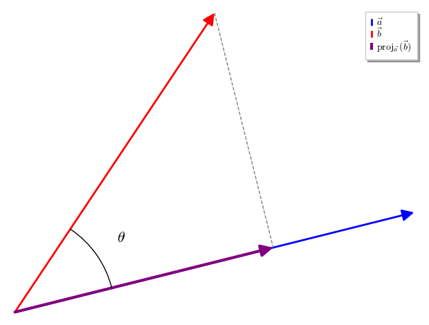
In physics and engineering, we often need to know how much of a force is acting in a specific direction. For example, if we pull a wagon at an angle, only the horizontal component of our pull actually moves the wagon forward. We can find this component by projecting one vector onto another (Stewart et al. 2020, 12.3, pp. 851).
There are two ways to describe a projection: as a scalar (the “length” of the shadow) or as a vector (the shadow itself).
Scalar Projection (Component): The scalar projection of \(\vec{b}\) onto \(\vec{a}\), denoted \(\operatorname{comp}_{\vec{a}}\left(\vec{b}\right)\), is the signed length of the shadow of \(\vec{b}\) cast onto the line containing \(\vec{a}\). Using trigonometry, this is \(\left\lVert \vec{b} \right\rVert\cos\theta\). Substituting our cosine formula gives: \[
\operatorname{comp}_{\vec{a}}\left(\vec{b}\right) = \frac{\vec{a} \cdot \vec{b}}{\left\lVert \vec{a} \right\rVert}.
\]
Vector Projection: To turn this length back into a vector pointing in the direction of \(\vec{a}\), we multiply the scalar projection by the unit vector \(\hat{a} = \frac{\vec{a}}{\left\lVert \vec{a} \right\rVert}\):