flowchart LR
  A("2(x-2) = 2λx <br> 2y = -10λy <br> x²-5y² = 1")
  A --> B("2(x-λx-2) = 0 <br> 2y (1+5λ) = 0 <br> x²-5y² = 1")
  B -->|"y=0"| C("2(x-λx-2) = 0 <br> x² = 1")
  B -->|"λ=-1/5"| D("2(6x/5-2) = 0 <br> x²-5y² = 1")
  C -->|"x=1"| E("-2(1+λ) = 0")
  C -->|"x=-1"| F("2(-3+λ) = 0")
  E --> G("(x,y,λ) = (1,0,-1)"):::solution
  F --> H("(x,y,λ) = (-1,0,3)"):::solution
  D --> I("x = 5/3 <br> 25/9-5y^2 = 1")
  I --> J("(x,y,λ) = (5/3, -4/(3√5), -1/5)"):::solution
  I --> K("(x,y,λ) = (5/3, 4/(3√5), -1/5)"):::solution
21 Lagrange Multipliers II
21.1 Lagrangian formulation
NoteRemark
The Lagrangian combines the objective function \(f\) and the constraint function \(g\):
\[\mathcal{L}(x_1,\dots,x_n,\lambda) = f(x_1,\dots,x_n) - \lambda ( g(x_1,\dots,x_n) - c ).\]
This auxiliary function is useful because its critical points encode the \(n+1\) Lagrange equations:
\[\nabla \mathcal{L} = \langle f_{x_1} - \lambda g_{x_1}, \cdots, f_{x_n} - \lambda g_{x_n}, c - g \rangle.\]
The critical points (the stationary points) of the Lagrangian are the solutions to our optimization problem.
TipMethod of Lagrange multipliers (Stewart et al. 2020, 14.8.1)
We want to optimize \(f(x_1,\dots,x_n)\) subject to a constraint \(g(x_1,\dots,x_n) = c\).
- Compute the gradient of the Lagrangian \(\mathcal{L}(x_1,\dots,x_n,\lambda) = f - \lambda (g-c)\),
- Set \(\nabla \mathcal{L} = 0\) (a system of equations) and solve to find its stationary points, and
- Plug the stationary points into \(f(x_1,\dots,x_n)\) to determine extreme values.
If you prefer to solve constrained optimization problems without using the Lagrangian formulation, that’s fine!
21.2 More examples
NoteExample: Find the nearest point on the hyperbola \(x^2 - 5 y^2 = 1\) to the point \(P = (2,0)\).
We take \(f(x,y) = (x - 2)^2 + y^2\) (since the square of a function, namely the distance function, will inherit its critical points), \(g(x,y) = x^2 - 5 y^2\), and \(c = 1\).
We can check our work with Sage, using the Lagrangian formulation to simplify writing down the equations.
var('x y λ')
f = (x - 2)^2 + y^2
g = x^2 - 5*y^2
c = 1

L(x,y,λ) = f - λ*(g-c)
gradL = list(L.gradient())

solutions = solve(gradL, [x, y, λ])
real_solutions = [sol for sol in solutions
    if all(eq.rhs() in RR for eq in sol)]

print("Stationary points:")
for sol in real_solutions:
    val = f.subs(sol)
    print(f"f = {val} when {sol}")
Stationary points:
f = 9 when [x == -1, y == 0, λ == 3]
f = 1 when [x == 1, y == 0, λ == -1]
f = 7/15 when [x == (5/3), y == 4/15*sqrt(5), λ == (-1/5)]
f = 7/15 when [x == (5/3), y == -4/15*sqrt(5), λ == (-1/5)]Writing list() in the above converts the result of L.gradient() into an object which Sage interprets as each entry as being set equal to \(0\). Regardless of how we solve, there are two absolute minima (\(f=\frac{7}{15}\)), and all are visualized below in red:
constraint_curve = implicit_plot(
  g == c,
  (x, -2.5, 2.5),
  (y, -2.5, 2.5),
  color='cyan',
  zorder=1
)
stationary_points = point([
  (x.subs(sol), y.subs(sol)) for sol in real_solutions],
  color='red',
  size=50,
  zorder=2
)
P = point((2,0), color='black', size=40)

show(constraint_curve + stationary_points + P)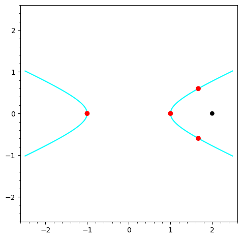
What is the significance of the points that did not give the absolute minimum?
NoteExample: extrema of \(f(x,y) = x y e^{-x^2 - y^2}\), subject to \(g(x,y) = 2 x - y\) and \(c = 0\).
Since the constraint is quite simple, we solve \(y = 2x\) and substitute into the other Lagrange equations: \[ e^{-5x^2} \langle 2x(2x^2-1), x(4x^2-1) \rangle = \lambda \langle 2, -1 \rangle. \] Solving for \(\lambda\) in both equations and equating gives \(x(2x^2-1) e^{-5x^2} = x(1-8x^2) e^{-5x^2}.\) Hence we have \[ x(2x^2-1) = x(1-8x^2) \implies 2 x (5 x^2 - 1) = 0 \implies x = 0 \text{ or } x = \pm \tfrac{1}{\sqrt{5}}. \] Thus the stationary points of the Lagrangian are: \[(0, 0, 0), (\tfrac{1}{\sqrt{5}}, \tfrac{2}{\sqrt{5}}, \tfrac{3}{5 \sqrt{5} e}), (-\tfrac{1}{\sqrt{5}}, -\tfrac{2}{\sqrt{5}}, -\tfrac{3}{5 \sqrt{5} e}).\] The first is the minimum (\(f=0\)) and the last two are maxima (\(f=\frac{2}{5e}\)).
21.3 Homework
- (Stewart et al. 2020, sec. 14.8) #41, 43–45, 47, 54–55
You should also reflect on the bonus problem, §14.8.35.