var('t y')
plot_slope_field(y - t, (t, -2, 2), (y, -2, 2), color='gray')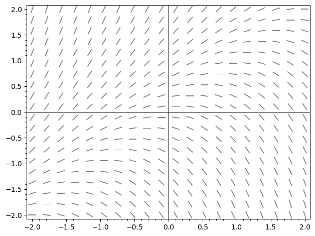
SageMath Spotlight
plot_slope_field(f(t,y), (t, t_min, t_max), (y, y_min, y_max))streamline_plot(f(t,y), (t, t_min, t_max), (y, y_min, y_max))A first-order differential equation takes the form \(\frac{\mathop{}\!\mathrm{d}y}{\mathop{}\!\mathrm{d}t} = f(t, y)\). This equation tells us the slope of the solution curve \(y(t)\) at any given coordinate \((t, y)\) in the plane. By drawing small line segments with the calculated slope at a grid of points, we can visualize the entire family of solutions without doing any calculus. This grid of slopes is called a slope field (or direction field).
If we drop a point onto this field and follow the arrows step-by-step, we trace out a solution curve to the differential equation (called an integral curve).
This slope-following process forms the foundation of Euler’s Method (Stewart et al. 2020, 9.2, pp. 616) for numerically approximating differential equations: measure the current slope, take a small step in that direction, re-evaluate the slope at the new position, and repeat. While numerical integration does not yield an exact symbolic formula, it can produce accurate numerical approximations for equations that cannot be solved by hand!
Example 8.1 Consider the differential equation \(y' = y - t\).
Plotting these tangent lines across a grid (at considerably more points) gives the slope field:
var('t y')
plot_slope_field(y - t, (t, -2, 2), (y, -2, 2), color='gray')
We can imagine dropping particles into a fluid flowing along these tangent directions and watching the trajectories they trace out. In SageMath, we overlay continuous flow lines onto the slope field using streamline_plot:
var('t y')
slope_field = plot_slope_field(y - t, (t, -2, 2), (y, -2, 2), color='gray')
flow_lines = streamline_plot(y - t, (t, -2, 2), (y, -2, 2), color='blue')
show(slope_field + flow_lines, axes_labels=['$t$', '$y$'], aspect_ratio=1)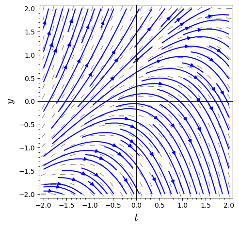
While slope fields provide qualitative insight, we often seek exact algebraic formulas. The simplest class of first-order differential equations to solve analytically are separable equations (Stewart et al. 2020, 9.3, pp. 621), which can be factored into a product of a function of \(y\) and a function of \(t\): \[ \frac{\mathop{}\!\mathrm{d}y}{\mathop{}\!\mathrm{d}t} = f(y) g(t). \]
Constant values \(y_0\) for which \(f(y_0) = 0\) are called equilibrium solutions (also, steady state solutions). These are solutions to the differential equation, since \(\frac{\mathop{}\!\mathrm{d}y}{\mathop{}\!\mathrm{d}t} = 0\) is true for the constant curve \(y(t) = y_0\).
We solve separable equations by algebraically isolating all \(y\) terms (including \(\mathop{}\!\mathrm{d}y\)) on one side and all \(t\) terms (including \(\mathop{}\!\mathrm{d}t\)) on the other, then integrating both sides: \[ \int \frac{1}{f(y)} \mathop{}\!\mathrm{d}y = \int g(t) \mathop{}\!\mathrm{d}t. \]
Example 8.2 (Stewart et al. (2020), chap. 9.3, pp. 622) Consider the differential equation \(\frac{\mathop{}\!\mathrm{d}y}{\mathop{}\!\mathrm{d}t} = \frac{t^2}{y^2}\), which separates to \[ y^2 \mathop{}\!\mathrm{d}y = t^2 \mathop{}\!\mathrm{d}t. \]
var('t y')
slope_field = plot_slope_field(t^2/y^2, (t, -2, 2), (y, -2, 2), color='gray')
flow_lines = streamline_plot(t^2/y^2, (t, -2, 2), (y, -2, 2), color='blue')
show(slope_field + flow_lines, axes_labels=['$t$', '$y$'], aspect_ratio=1)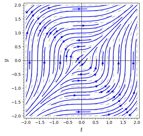
Integrating gives \(\frac{1}{3} y^3 = \frac{1}{3} t^3 + C\), or the simpler \[ y^3 = t^3 + C. \] Note that we have relabeled \(3C\) as \(C\), since the constant is arbitrary (as in Remark 4.1). Thus: \[ y = \sqrt[3]{t^3+C} \] is the general solution of our differential equation. There are no equilibrium solutions!
Example 8.3 (Radioactive Decay) The rate at which a radioactive substance decays is proportional to the current mass of the material: \(\frac{\mathop{}\!\mathrm{d}y}{\mathop{}\!\mathrm{d}t} = -ky\), where \(k > 0\) is the decay constant. Separating variables yields: \[ \begin{aligned} \frac{1}{y} \mathop{}\!\mathrm{d}y &= -k \mathop{}\!\mathrm{d}t \\ \int \frac{1}{y} \mathop{}\!\mathrm{d}y &= \int -k \mathop{}\!\mathrm{d}t \\ \ln\vert{}y\vert{} &= -kt + C. \end{aligned} \] Exponentiating both sides gives \(\vert{}y\vert{} = e^{-kt+C} = e^C e^{-kt}\). Letting \(A = \pm e^C\) (or \(0\)), we recover the standard exponential model: \[ y(t) = A e^{-kt}. \] If we specify an initial condition \(y(0) = y_0\), then \(A = y_0\) gives the trajectory \(y(t) = y_0 e^{-kt}\).
Note that \(y(t) = 0\) is the only equilibrium solution to this differential equation. What does it physically represent?
Example 8.4 (Reaction Kinetics and \(n\)th-Order Rates) In chemistry, the rate at which a reactant \(A\) with concentration \(y(t) = [A]\) is consumed in an \(n\)th-order reaction is governed by the differential equation: \[ \frac{\mathop{}\!\mathrm{d}y}{\mathop{}\!\mathrm{d}t} = -k y^n \quad (k > 0). \] The order \(n\) dictates how concentration scales over time:
Again, \(y(t) = 0\) is the only equilibrium solution.
In experimental chemistry, determining the rate order \(n\) of a reaction is often done by measuring concentration \(y(t)\) over time:
These graphical diagnostics exist precisely because they are the integrated solutions to separable differential equations!
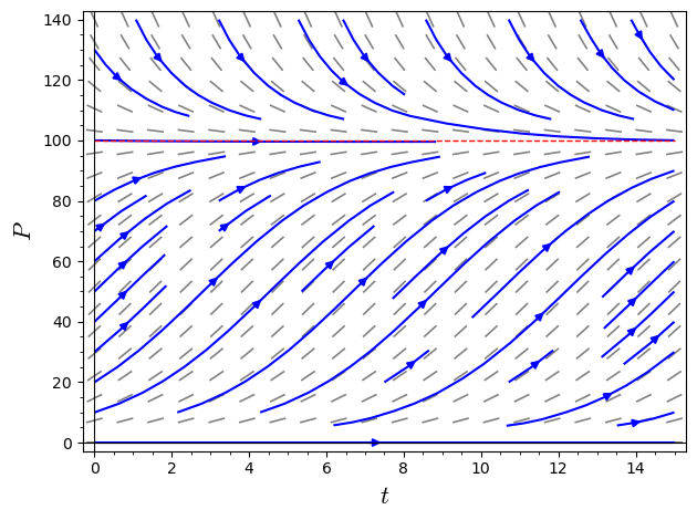
Example 8.5 (Logistic Population Growth (Stewart et al. 2020, 9.4, pp. 632)) Unconstrained growth \(\frac{\mathop{}\!\mathrm{d}P}{\mathop{}\!\mathrm{d}t} = kP\) predicts that populations grow infinitely. A more realistic model incorporates an environmental carrying capacity \(M\), slowing growth as the population approaches resource limits: \[ \frac{\mathop{}\!\mathrm{d}P}{\mathop{}\!\mathrm{d}t} = k P \left(1 - \frac{P}{M}\right). \] This equation is separable: \[ \int \frac{1}{P\left(1 - \frac{P}{M}\right)} \mathop{}\!\mathrm{d}P = \int k \mathop{}\!\mathrm{d}t. \] To evaluate the left-hand integral, we use partial fraction decomposition (Section 5.3): \[ \frac{1}{P\left(1 - \frac{P}{M}\right)} = \frac{1}{P} + \frac{1/M}{1 - P/M}. \] Integrating both terms yields: \[ \begin{aligned} \int \left( \frac{1}{P} + \frac{1/M}{1 - P/M} \right) \mathop{}\!\mathrm{d}P &= \int k \mathop{}\!\mathrm{d}t \\ \ln\vert{}P\vert{} - \ln\left|1 - \frac{P}{M}\right| &= kt + C \\ \ln\left| \frac{P}{1 - P/M} \right| &= kt + C. \end{aligned} \] Exponentiating both sides yields \(\frac{P}{1 - P/M} = C_1 e^{kt}\). Solving for \(P(t)\): \[ P(1 - P/M)^{-1} = C_1 e^{kt} \implies P = C_1 e^{kt} \left(1 - \frac{P}{M}\right). \] Algebraically rearranging to isolate \(P(t)\) gives the logistic curve: \[ P(t) = \frac{M}{1 + A e^{-kt}}, \] where \(A = \frac{M - P_0}{P_0}\) is determined by the initial population \(P(0) = P_0\).
We have two equilibrium solutions: \(y(t) = 0\) and \(y(t) = M\). What do they represent?
Notice that if \(0 < P_0 < \frac{1}{2} M\), the trajectory forms a classic “S-curve” that grows exponentially at first, passes an inflection point, and asymptotically approaches \(M\) as \(t \to \infty\).
var('t P')
k = 0.5
M = 100
f = k * P * (1 - P/M)

slope_field = plot_slope_field(
    f,
    (t, 0, 15), (P, 0, 140),
    color='gray'
)
flow_lines = streamline_plot(
    f,
    (t, 0, 15), (P, 0, 140),
    color='blue', density=0.5
)
capacity_line = plot(
    M,
    (t, 0, 15),
    color='red', linestyle='--'
)

show(slope_field + flow_lines + capacity_line, axes_labels=['$t$', '$P$'])