1 Review
1.1 Limits
Calculus is the mathematics of motion and change. To make sense of change at a single instant, we need a systematic way to speak of vanishingly small quantities—this is how we arrive at the subtle and ethereal notion of limits which are central to modern mathematics.
Notion of Limit (Stewart et al. 2020, 2.2.1, pp. 83)
The limit of \(f(x)\) at \(x=a\), when it exists, is the value \(L\) that \(f(x)\) approaches as the argument \(x\) gets arbitrarily close to (but not equal to!) \(x=a\). In such a situation, we write \[ L = \lim_{x \to a} f(x). \] If we also have that \(L = f(a)\), then \(f(x)\) is continuous at \(x=a\); otherwise, \(f(x)\) is discontinuous at \(x=a\). A function is continuous if it is continuous at each point in its domain.
It is perfectly reasonable to speak about a limit of a function being infinite (either \(\infty\) or \(-\infty\)) at a given point if \(f(x)\) grows arbitrarily large or arbitrarily negative when \(x\) is sufficiently close to (but not equal to!) \(a\). We write \[ \lim_{x \to a} f(x) = \infty, \] but remember that this is notation—we don’t mean to suggest that \(\infty\) is a number!
Most of the functions we will study in this course are continuous or, at worst, discontinuous in only a handful of places!
One-Sided Limits
For a limit to exist, all ways of approaching \(a\) for values of \(x\) in the domain of the function should approach the same value \(L\). This is not always the case!
Notion of One-Sided Limits (Stewart et al. 2020, 2.2.2, pp. 86)
The left-hand limit of \(f(x)\) at \(x=a\) is the value \(L\) that \(f(x)\) approaches as we move \(x\) toward \(a\) from the left (\(x < a\)). In such a situation, we write \[ L = \lim_{x \to a^-} f(x). \] We also have the right-hand limit of \(f(x)\), which is the value \(M\) that \(f(x)\) approaches as we move \(x\) toward \(a\) from the right (\(x > a\)), written \[ M = \lim_{x \to a^+} f(x). \]
Existence of Limits (Stewart et al. 2020, 2.2.3, pp. 87)
The limit of a function \(f(x)\) at \(x=a\) exists if and only if the one-sided limits of \(f(x)\) exist at \(x=a\) and are equal, in which case we have \[ \lim_{x \to a} f(x) = \lim_{x \to a^+} f(x) = \lim_{x \to a^-} f(x). \]
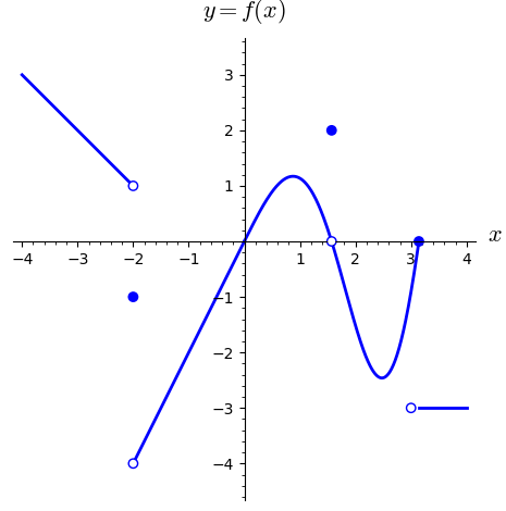
Example 1.1 (Some functions) Here we demonstrate behaviors which illustrates the sorts of functions we will encounter in this course.
At the discontinuities, we have the following limits and values:
\[ \begin{aligned} \lim_{x \to -2^-} f(x) & = 1 & \qquad & & f(-2) & = -1 & \qquad & & \lim_{x \to -2^+} f(x) & = -4 \\ \lim_{x \to \frac{\pi}{2}} f(x) & = 0 & & & f(\tfrac{\pi}{2}) & = 2 \\ \lim_{x \to \pi^-} f(x) = f(\pi) & = 0 & & & \lim_{x \to \pi^+} f(x) & = -3 \\ \end{aligned} \]
We will not be too concerned with the distinctions in this class, but many pre-calculus courses talk about the discontinuity at \(x=\frac{\pi}{2}\) as being removable (whereas the other two are essential) because we can repair the continuity of \(f(x)\) by changing its value in this one place.
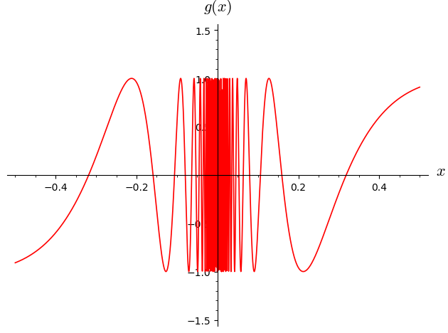
On the other hand, some functions have points which do not admit a left or right limit at all:
Limits at Infinity
Limits can also be used to ask: “What happens to our function as \(x\) grows arbitrarily large?” Visually, these limits describe the horizontal asymptotes of a graph.
Notion of Limits at Infinity (Stewart et al. 2020, 2.6.1, pp. 127)
If the values of \(f(x)\) become arbitrarily close to a single number \(L\) as \(x\) grows larger and larger without bound in the positive direction, we write
\[ \lim_{x \to \infty} f(x) = L. \]
Similarly, if \(f(x)\) approaches a number \(M\) as \(x\) moves indefinitely far out in the negative direction, we write
\[ \lim_{x \to -\infty} f(x) = M. \]
Example 1.2 Consider the following:
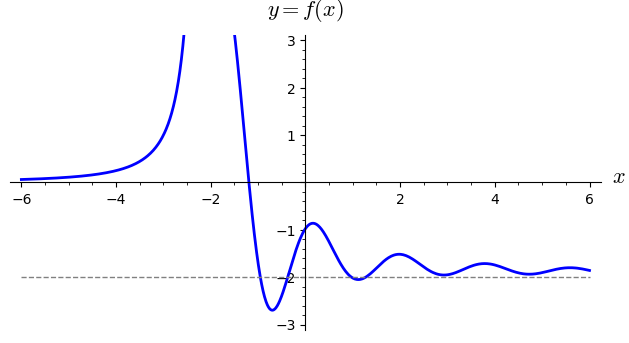
Looking at the graph, as we trace the curve further and further to the left or right, it flattens out and gets closer and closer to values \(y=0\) and \(y=-2\), respectively. We have:
\[ \lim_{x \to -\infty} f(x) = 0 \quad \text{and} \quad \lim_{x \to \infty} f(x) = -2. \]
Properties of Limits
Limits, when they exist, are well-behaved—they satisfy a collection of properties that match exactly how we might hope they work. Essentially, as long as we are careful to avoid illegal operations (like dividing by zero), the limit of a combination of functions is just the combination of their individual limits!
Properties of Limits (Stewart et al. 2020, 2.3, pp. 95)
Suppose that \(\displaystyle \lim_{x \to a} f(x) = L\) and \(\displaystyle \lim_{x \to a} g(x) = M\), where \(L\) and \(M\) are real numbers. Then:
- Homogeneity: For any real number \(c\), we have \(\displaystyle \lim_{x \to a} \left( c\ f(x) \right) = c\ L\)
- Additivity: \(\displaystyle \lim_{x \to a} \left( f(x) \pm g(x) \right) = L \pm M\)
- Product Law: \(\displaystyle \lim_{x \to a} (f(x)\ g(x)) = L\ M\)
- Quotient Law: So long as \(M \not = 0\), we have \(\displaystyle \lim_{x \to a} \frac{f(x)}{g(x)} = \frac{L}{M}\)
- Power Law: For any number \(c > 0\), we have \(\displaystyle \lim_{x \to a} \left( f(x) \right)^c = L^c\)
Moreover, \(\displaystyle \lim_{x \to a} c = c\) and \(\displaystyle \lim_{x \to a} x = a\) for all real numbers \(a\) and \(c\).
Because of these properties, limits of well-behaved continuous expressions (like polynomials, terms involving \(\sin(x)\) and \(\cos(x)\), compositions therein, etc.) are as simple as direct substitution: we can just plug \(x=a\) straight into the formula!
Euler’s Number
An important constant in calculus, Euler’s number (written as the letter \(e\)), arises from the study of limits.
Definition 1.1 (Definition of \(e\)) \[ e \coloneqq \lim_{n \to \infty} \left( 1 + \frac{1}{n} \right)^n \approx 2.718281828459\dots. \]
Like many concepts in modern mathematics, Euler’s number was developed through applications to finance. Imagine we have \(\$1\) in a bank account that pays a \(100\%\) interest rate (this will, of course, never happen).
- If the bank compounds our interest once a year (\(n=1\)), we have \((1 + \frac{1}{1})^1 = \$2.00\) at the end of the year.
- If they compound twice a year (\(n=2\)), we get \(50\%\) halfway through and \(50\%\) (of the increased amount!) at the end, yielding \((1 + \frac{1}{2})^2 = \$2.25\).
- If they compound daily (\(n=365\)), we end up with \((1 + \frac{1}{365})^{365} \approx \$2.71456748\dots\).
What if the bank compounds our interest every hour? Every second? Can we speak of instantaneously compounding interest? Indeed, as \(n \to \infty\), our money limits towards \(e\).
1.2 Derivatives
Derivatives are a special kind of limit which allow us to study the local behavior of a function. Geometrically, the derivative measures the steepness of a curve; physically, it represents an instantaneous rate of change.
As Limits
The Derivative as a Limit (Stewart et al. 2020, 2.8, pp. 153)
If \(f(x)\) is a continuous function at a number \(x=a\) and the limit
\[ \lim_{h \to 0} \frac{f(a+h)-f(a)}{h} \]
exists, then it is called the derivative of \(f(x)\) at \(x=a\) and denoted \(f'(a)\); we say that \(f(x)\) is differentiable at \(x=a\). The function
\[ f'(x) \coloneqq \lim_{h \to 0} \frac{f(x+h)-f(x)}{h}, \]
defined wherever \(f(x)\) is differentiable, is called the derivative of \(f(x)\).
Notation
We also use Leibniz notation for derivatives, writing \(\frac{\mathop{}\!\mathrm{d}f}{\mathop{}\!\mathrm{d}x}\) or \(\frac{\mathop{}\!\mathrm{d}}{\mathop{}\!\mathrm{d}x}f(x)\) for the quantity \(f'(x)\) described above.
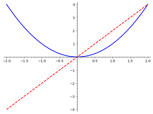
Example 1.3 Consider \(f(x) = x^2\). We compute
\[ \begin{aligned} f'(x) & = \lim_{h \to 0} \frac{(x+h)^2-x^2}{h} \\ & = \lim_{h \to 0} \frac{x^2+2xh+h^2-x^2}{h} \\ & = \lim_{h \to 0} (2x + h) \\ & = 2x. \end{aligned} \]
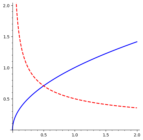
Example 1.4 Consider \(f(x) = \sqrt{x}\). We compute
\[ \begin{aligned} f'(x) & = \lim_{h \to 0} \frac{\sqrt{x+h}-\sqrt{x}}{h} \\ & = \lim_{h \to 0} \frac{\sqrt{x+h}-\sqrt{x}}{h} \frac{\sqrt{x+h}+\sqrt{x}}{\sqrt{x+h}+\sqrt{x}} \\ & = \lim_{h \to 0} \frac{(x+h)-x}{h} \frac{1}{\sqrt{x+h}+\sqrt{x}} \\ & = \lim_{h \to 0} \frac{1}{\sqrt{x+h}+\sqrt{x}} \\ & = \frac{1}{2\sqrt{x}}. \end{aligned} \]
As Tangents
Geometrically, the secant line connecting two points on a curve approaches a unique limiting line as those points are brought infinitely close together. This limiting line is the tangent line, and its slope at that spot is given by the derivative.
The Tangent Line (Stewart et al. 2020, 2.7, pp. 145)
If \(f(x)\) is differentiable at \(x=a\), then the line given by \[ y = f'(a) (x-a) + f(a) \] is called the tangent line to \(f(x)\) at \(x=a\).
Fermat’s Theorem (Stewart et al. 2020, 4.1, pp. 282)
If \(f(x)\) has a local maximum or local minimum at \(x=c\), and if \(f'(c)\) exists, then \(f'(c) = 0\).
Geometrically, this means the tangent line to the curve at a peak or a valley is horizontal.
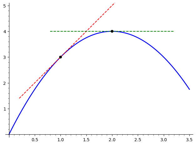
Example 1.5 Consider the function \(f(x) = -x^2 + 4x\). Its derivative is \(f'(x) = -2x + 4\).
- At \(x = 1\), the slope of the curve is \(f'(1) = 2\). Since \(f(1) = 3\), the equation of the tangent line is \(y = 2(x-1) + 3\), or \(y = 2x + 1\).
- At \(x = 2\), the slope of the curve is \(f'(2) = 0\). Since this derivative vanishes, we identify a local maximum at the point \((2,4)\), where the tangent line is the horizontal line \(y = 4\).
Elementary Functions
We rarely compute derivatives in terms of limits! Instead, having worked out the derivatives for some common functions, we rely on a variety of techniques that allow us to find derivatives of more complicated expressions built from them.
Linearity of the Derivative (Stewart et al. 2020, 3.1, pp. 177)
Let \(f(x)\) and \(g(x)\) be differentiable functions, and let \(c\) be any constant real number. Then:
- Homogeneity: \(\displaystyle \frac{\mathop{}\!\mathrm{d}}{\mathop{}\!\mathrm{d}x} \left( c\ f(x) \right) = c\ f'(x)\)
- Additivity: \(\displaystyle \frac{\mathop{}\!\mathrm{d}}{\mathop{}\!\mathrm{d}x} \left( f(x) \pm g(x) \right) = f'(x) \pm g'(x)\)
Moreover, \(\displaystyle \frac{\mathop{}\!\mathrm{d}}{\mathop{}\!\mathrm{d}x} c = 0\) and \(\displaystyle \frac{\mathop{}\!\mathrm{d}}{\mathop{}\!\mathrm{d}x} x = 1\) for all real numbers \(c\).
Polynomials
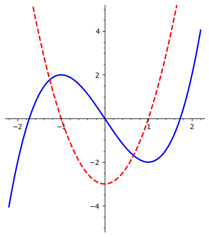
The foundational shortcut for algebraic functions is the Power Rule. Combined with the previous fact that derivatives distribute over addition and pass through constants, we can differentiate any polynomial term-by-term.
The Power Rule (Stewart et al. 2020, 3.1, pp. 176)
For any real number \(n\):
\[ \frac{\mathop{}\!\mathrm{d}}{\mathop{}\!\mathrm{d}x} \left(x^n\right) = n x^{n-1}. \]
Exponentials
Exponential functions grow at a rate directly proportional to their current magnitude. In particular, one of the reasons Euler’s number \(e\) is so special is that \(e^x\) is a very special function—it is equal to its own derivative!
Derivatives of Exponentials (Stewart et al. 2020, 3.1, pp. 180)
\[ \frac{\mathop{}\!\mathrm{d}}{\mathop{}\!\mathrm{d}x}\left( e^x \right) = e^x. \]
Trigonometric
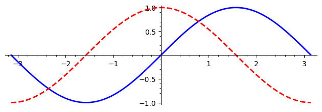
Trigonometric derivatives describe the periodic, oscillating rates of change found within circular geometric motions.
Common Trigonometric Derivatives (Stewart et al. 2020, 3.3, pp. 193)
\[ \frac{\mathop{}\!\mathrm{d}}{\mathop{}\!\mathrm{d}x}\left( \sin x \right) = \cos x, \qquad \frac{\mathop{}\!\mathrm{d}}{\mathop{}\!\mathrm{d}x}\left( \cos x \right) = -\sin x, \qquad \frac{\mathop{}\!\mathrm{d}}{\mathop{}\!\mathrm{d}x}\left( \tan x \right) = \sec^2 x. \]
Product and Quotient Rules
When separate functions are bound together via multiplication or division, their individual rates of change interact in non-trivial ways. We cannot simply multiply or divide the underlying derivatives!
Product and Quotient Rules (Stewart et al. 2020, 3.2, pp. 185)
If \(f\) and \(g\) are differentiable functions, then:
- Product Rule: \(\frac{\mathop{}\!\mathrm{d}}{\mathop{}\!\mathrm{d}x}[f(x)g(x)] = f'(x)g(x) + f(x)g'(x)\)
- Quotient Rule: \(\frac{\mathop{}\!\mathrm{d}}{\mathop{}\!\mathrm{d}x}\left(\frac{f(x)}{g(x)}\right) = \frac{f'(x)g(x) - f(x)g'(x)}{[g(x)]^2}\) (where \(g(x) \neq 0\))
The Chain Rule
To find the rate of change of a composite function (a function nested inside another expression), we track variations from the outside in. The heuristic is to differentiate the outer wrapper while keeping the inner expression intact, then scale our result by the derivative of that inner expression.
The Chain Rule (Stewart et al. 2020, 3.4, pp. 200)
If \(g\) is differentiable at \(a\) and \(f\) is differentiable at \(g(a)\), then the composite function \(F(x) = f(g(x))\) is differentiable at \(a\). In general, the derivative of the composite is given by
\[ F'(x) = f'(g(x))\ g'(x). \]
Implicit Differentiation
Not all mathematical correspondences can be easily pulled apart into an explicit equation \(y = f(x)\). Even when variables are related only implicitly, we can still study the way these quantities change (\(\frac{\mathop{}\!\mathrm{d}y}{\mathop{}\!\mathrm{d}x}\)) by taking the derivative of both sides with respect to \(x\)—keeping in mind that \(y\) is a function of \(x\), which requires an application of the Chain Rule.
Logarithms
By writing the logarithmic expression \(y = \ln x\) in its implicit exponential form \(e^y = x\) and differentiating implicitly, we can find the rate of change for natural logarithmic fields.
Derivatives of Logarithms (Stewart et al. 2020, 3.6, pp. 218)
\[ \frac{\mathop{}\!\mathrm{d}}{\mathop{}\!\mathrm{d}x} \left( \ln x \right) = \frac{1}{x}. \]
Inverse Trigonometric Functions
Similarly, applying implicit differentiation to formal trigonometric inverses (for example, rewriting \(y = \arctan x\) as \(\tan y = x\)) yields the following:
Inverse Trigonometric Derivatives (Stewart et al. 2020, 3.6, pp. 222)
\[\frac{\mathop{}\!\mathrm{d}}{\mathop{}\!\mathrm{d}x} \arcsin x = \frac{1}{\sqrt{1-x^2}}, \qquad \frac{\mathop{}\!\mathrm{d}}{\mathop{}\!\mathrm{d}x}\arccos x = -\frac{1}{\sqrt{1-x^2}}, \qquad \frac{\mathop{}\!\mathrm{d}}{\mathop{}\!\mathrm{d}x} \arctan x = \frac{1}{1+x^2}.\]
1.3 Integrals and Antiderivatives
Differentiation asks how a function changes, while integration asks how it accumulates. In particular, the fundamental theorem of calculus quantifies how these processes are inverse to one another!
Definite Integrals
The definite integral measures the net signed area bounded between a curve and the horizontal coordinate axis over some interval.
The Definite Integral (Stewart et al. 2020, 5.2.2, pp. 384)
The definite integral of a continuous function \(f(x)\) from \(x=a\) to \(x=b\) is defined as the limit of its Riemann sums as the width of the subintervals approaches zero:
\[\int_{a}^{b} f(x) \mathop{}\!\mathrm{d}x = \lim_{n \to \infty} \sum_{i=1}^{n} f(x_i^*) \, \Delta x.\]
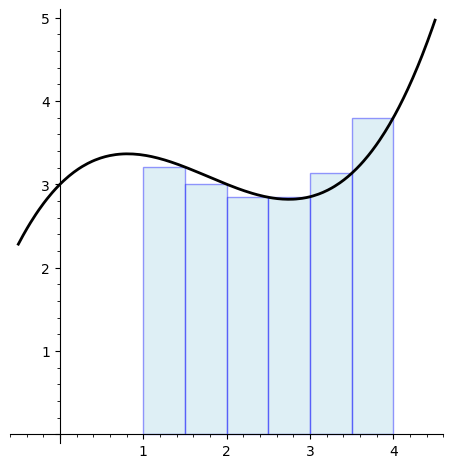
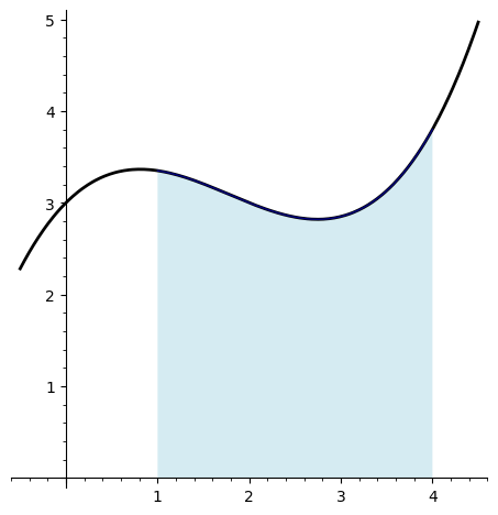
Before passing to the infinite limit that defines the exact area under a curve, we approximate the region using a finite collection of rectangles. As the number of rectangles \(n\) grows large, the width \(\Delta x\) vanishes, smoothing our discrete blocks into a continuous calculation of net area.
The Fundamental Theorem of Calculus
The Fundamental Theorem of Calculus (Stewart et al. 2020, 5.3, pp. 399)
Suppose \(f\) is continuous on \([a, b]\).
- If \(g(x) = \displaystyle \int_{a}^{x} f(t) \mathop{}\!\mathrm{d}t\), then \(g'(x) = f(x)\).
- If \(F\) is an antiderivative of \(f\) (i.e., \(F' = f\)), then \(\displaystyle \int_{a}^{b} f(x) \mathop{}\!\mathrm{d}x = F(b) - F(a)\).
In other words, integrals (areas under curves) can be computed by reversing the process of differentiation. Just as with derivatives, we will not use Riemann sums to compute integrals in this course! Instead, we will rely on the fundamental theorem of calculus, together with various techniques for computing antiderivatives.
Elementary Antiderivatives
Just as we developed shortcuts to avoid computing derivatives using limits, we can reverse those rules to find general antiderivatives (without computing Riemann sums):
- Reverse Power Rule: \(\displaystyle \int x^n \mathop{}\!\mathrm{d}x = \frac{x^{n+1}}{n+1} + C\) (for \(n \neq -1\))
- Logarithm Rule: \(\displaystyle \int \frac{1}{x} \mathop{}\!\mathrm{d}x = \ln|x| + C\)
- Exponential Rule: \(\displaystyle \int e^x \mathop{}\!\mathrm{d}x = e^x + C\)
- Trigonometric Rules: \(\displaystyle \int \cos x \mathop{}\!\mathrm{d}x = \sin x + C\) and \(\displaystyle \int \sin x \mathop{}\!\mathrm{d}x = -\cos x + C\)
\(u\)-Substitution
The Substitution Rule is the integration technique which arises from applying the Chain Rule in reverse.
When looking at a complex integral, we seek to identify an “inner” functional expression \(g(x)\) whose corresponding differential scaling factor \(g'(x) \mathop{}\!\mathrm{d}x\) is also actively present within the integrand. By changing our coordinates into this temporary \(u\)-space, we can simplify a daunting expression into an elementary pattern that we already know how to integrate.
The Substitution Rule (Stewart et al. 2020, 5.5, pp. 420)
If \(u = g(x)\) is a differentiable function whose range is an interval \(I\), and \(f\) is continuous on \(I\), then:
\[ \int f(g(x)) \, g'(x) \mathop{}\!\mathrm{d}x = \int f(u) \mathop{}\!\mathrm{d}u. \]
Example 1.6 Consider the indefinite integral
\[ \int 2x \, e^{x^2} \mathop{}\!\mathrm{d}x. \]
We notice that the nested exponent expression is \(u = x^2\), and its derivative \(2x\) is multiplying the rest of the integrand (\(\mathop{}\!\mathrm{d}u = 2x \mathop{}\!\mathrm{d}x\)). Substituting these elements into our original integral simplifies the problem:
\[ \int e^{x^2} \left( 2x \mathop{}\!\mathrm{d}x \right) = \int e^{u} \mathop{}\!\mathrm{d}u = e^u + C. \]
Returning to our original coordinates gives us our final family of antiderivatives: \(e^{x^2} + C\).