t = var('t')
y(t) = 5 * exp(-2*t)

if diff(y(t), t) + 2*y(t) == 0:
    print(f"{y(t)} IS a solution!")
    show(plot(y(t), (t, 0, 2)))
else:
    print(f"{y(t)} is NOT a solution!")
5*e^(-2*t) IS a solution!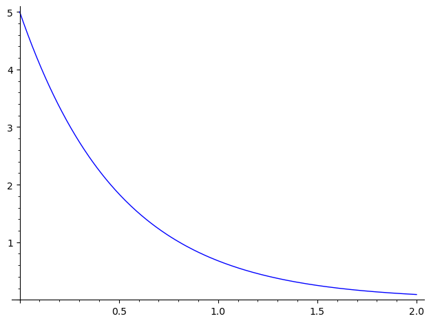
SageMath Spotlight
==if and elset = var('t')y = function('y')(t)diff(y(t), t)diff(y(t), t, 2)Algebra courses are often the first context in which we take observations about the world and systematically deduce properties from them. Beginning with a statement like “the area plus twice the side length of a square is 10,” we write down an algebraic equation (\(x^2 + 2x = 10\)) and solve it, determining which numbers satisfy the relationship: \[ x^2 + 2x = 10 \implies x = -4.3166\dots \text{ and } 2.3166\dots. \] From here, we make judgments about how the quantities we have computed relate to reality (e.g., the square in question must have a positive side length, so we discard the negative root).
While this quantitative framework is useful for static problems, natural and social phenomena rarely stand still! Scientific inquiry has relied on different paradigms over the last two hundred years: rather than measuring static states, we formulate rules about how quantities change relative to one another. In this sense, differential equations are a framework for formalizing hypothetical mechanisms of change: when we construct a model, we encode a hypothesis about local rates of change and solve it to deduce the global trajectories that such rules permit.
Differential Equations and Solutions
A differential equation (DE) is an equation involving unknown functions \(y(t)\) and their derivatives \(y', y'', \dots, y^{(n)}\). Sometimes differential equations might involve many functions, perhaps dependent on one another and more generalized notions of derivatives, though we will restrict our attention to single functions varying with respect to some independent parameter. The order of a differential equation is the highest derivative which appears in it.
A function \(y = y(t)\) is a solution to a differential equation if substituting \(y\) and its derivatives into the equation yields a statement that is identically true for all \(t\) in its domain.
We emphasize that while solving algebraic equations yields static numbers, solutions to differential equations are functions, trajectories, or curves.
Example 7.1 (\(y(t) = 5 e^{-2t}\) as a solution to \(\frac{\mathop{}\!\mathrm{d}y}{\mathop{}\!\mathrm{d}t} + 2y = 0\)) By substitution, we will verify that \(y(t) = 5 e^{-2t}\) solves the equation \(y'+2y=0\). First, we compute the derivative of our candidate function: \[ \frac{\mathop{}\!\mathrm{d}y}{\mathop{}\!\mathrm{d}t} = \frac{\mathop{}\!\mathrm{d}}{\mathop{}\!\mathrm{d}t}\left(5 e^{-2t}\right) = -10 e^{-2t}. \] Next, we substitute \(y(t)\) and \(\frac{\mathop{}\!\mathrm{d}y}{\mathop{}\!\mathrm{d}t}\) into the left-hand side of the differential equation: \[ \frac{\mathop{}\!\mathrm{d}y}{\mathop{}\!\mathrm{d}t} + 2y = \left(-10 e^{-2t}\right) + 2\left(5 e^{-2t}\right) = -10 e^{-2t} + 10 e^{-2t} = 0. \] Because the left-hand side reduces identically to \(0\), \(y(t) = 5 e^{-2t}\) is indeed a solution.
We can also verify in SageMath:
t = var('t')
y(t) = 5 * exp(-2*t)
if diff(y(t), t) + 2*y(t) == 0:
print(f"{y(t)} IS a solution!")
show(plot(y(t), (t, 0, 2)))
else:
print(f"{y(t)} is NOT a solution!")5*e^(-2*t) IS a solution!
Example 7.2 (\(y(t) = \cos(3t) - 2\sin(3t)\) as a solution to \(\frac{\mathop{}\!\mathrm{d}^{2}y}{\mathop{}\!\mathrm{d}t^{2}} + 9y = 0\)) As above, we verify a solution to the second-order equation \(y'' + 9y = 0\). We compute the first and second derivatives: \[ \begin{aligned} y'(t) &= -3\sin(3t) - 6\cos(3t), \\ y''(t) &= -9\cos(3t) + 18\sin(3t). \end{aligned} \] Substituting \(y''(t)\) and \(y(t)\) into the left-hand side yields: \[ y'' + 9y = \big(-9\cos(3t) + 18\sin(3t)\big) + 9\big(\cos(3t) - 2\sin(3t)\big) = 0. \] The equation balances, so \(y(t) = \cos(3t) - 2\sin(3t)\) is a solution.
Notice that in Example 7.1, \(y(t) = 5e^{-2t}\) was not the only function that could satisfy \(y' + 2y = 0\). Indeed, any function of the form \(y(t) = C e^{-2t}\) (for any constant \(C\)) yields a valid solution. In a differential equations course, one can prove these are all the solutions to the equation: the general solution.1 Because integration is fundamentally involved in reversing differentiation, arbitrary constants naturally arise. Consequently, a differential equation on its own does not describe a single trajectory, but rather infinite families of solutions.
To isolate a single trajectory from this infinite family, we need additional information: an initial condition that specifies the state of the system at a particular moment. This fits into another important part of modern scientific paradigms: to understand a system, we need to know the rules that govern it, but also its initial state.
Initial Value Problem (IVP)
An Initial Value Problem consists of a differential equation together with a set of initial conditions. For our purposes, these will be of the form: \[ \frac{\mathop{}\!\mathrm{d}y}{\mathop{}\!\mathrm{d}t} = f(t, y), \quad y(t_0) = y_0. \] Solving an IVP means finding the unique particular solution from the general family that passes through the specified point \((t_0, y_0)\).
Example 7.3 (Constant Acceleration under Gravity) Consider an object falling near Earth’s surface. Repeated experiments have demonstrated that free-falling objects accelerate towards the surface of the earth at a rate of 9.8 meters per second squared. We can model the height \(y(t)\) of a free-falling particle (neglecting drag) with a second-order differential equation: \[ \frac{\mathop{}\!\mathrm{d}^{2}y}{\mathop{}\!\mathrm{d}t^{2}} = -9.8. \] Integrating once with respect to time yields the velocity of the particle: \[ \frac{\mathop{}\!\mathrm{d}y}{\mathop{}\!\mathrm{d}t} = -9.8t + v_0, \] where \(v_0\) is its initial velocity. Integrating a second time yields the position of the particle (the general solution of the original differential equation): \[ y(t) = -4.9t^2 + v_0 t + y_0. \] Here \(v_0\) and \(y_0\) are the initial velocity \(y'(0)\) and initial height \(y(0)\). Specifying these parameters (e.g., \(y(0) = 100\) meters and \(y'(0) = 0\) m/s) selects a unique trajectory out of the family, from which we can model a given physical scenario.
Sometimes we can identify solutions simply by asking structural questions about functions and their derivatives.
Example 7.4 (Unconstrained Population Growth (Stewart et al. 2020, 9.4, pp. 631)) Suppose we observe a bacterial colony, watching how each bacterium splits into more bacteria. We might hypothesize that “the rate of population growth is directly proportional to the current population size.” We write: \[ \frac{\mathop{}\!\mathrm{d}P}{\mathop{}\!\mathrm{d}t} = k P, \] where \(k\) is a positive constant. Instead of applying technical steps, we can ask: What family of functions is proportional to its own first derivative? After some reckoning with our intuition, we recall that exponential functions \(e^{kt}\) fit the bill! Thus, the general solution is: \[ P(t) = P_0 e^{kt}, \] where \(P_0 = P(0)\) represents the initial population at time \(t = 0\).
Example 7.5 (Hooke’s Law and Simple Harmonic Motion) Connecting a mass to a spring creates a restoring force proportional to displacement (\(F = -kx\)). By Newton’s second law, the position \(x(t)\) satisfies: \[ \frac{\mathop{}\!\mathrm{d}^{2}x}{\mathop{}\!\mathrm{d}t^{2}} = -\frac{k}{m} x. \] Asking what functions are equal to their own negative second derivative leads directly to sine and cosine. Setting \(\omega = \sqrt{k/m}\), any combination of the form: \[ x(t) = C_1 \cos(\omega t) + C_2 \sin(\omega t) \] will satisfy the differential equation. The constants \(C_1\) and \(C_2\) are determined by the initial position and initial velocity of the mass.
Below are two simulations of physical systems governed by simple differential equations—we can adjust their parameters to observe how local rules give rise to intricate global behavior!
Note how slighly different configurations of the mass lead to completely different trajectories! This is an example of chaos emerging from dynamical systems.
The mathematical principles of stability and synchronization have dramatic physical consequences!
This physical demonstration perfectly mirrors the mathematical behavior in the applet above!
A classic example of aeroelastic flutter, where wind created a runaway feedback loop of structural resonance.
When the bridge first opened in 2000, the natural gait of pedestrians synchronized with the bridge’s sway and caused an alarming feedback loop.
It is for this reason that we insist on writing the customary \(+C\) when evaluating an integral \(\int f(x) \mathop{}\!\mathrm{d}x\). After all, computing an indefinite integral is the same as describing all solutions of the equation \(\frac{\mathop{}\!\mathrm{d}x}{\mathop{}\!\mathrm{d}t} = f(x)\)!↩︎