19 Lagrange multipliers I

The second derivative test allows us to identify local maxima and minima of a function \(f(x,y)\) (this is often called optimization). The main goal of today is to solve a different, but related problem:

Goal

We want to optimize a function of two variables, \(f(x,y)\), (or maybe even a function of more variables, like \(f(x,y,z)\) or \(f(x_1,\dots,x_n)\)) but we are subject to a constraint \(g(x,y)=c\). We call \(f\) the objective function and \(g\) the constraint function.

In other words, we want to figure out how to make \(f(x,y)\) as large as possible (or as small as possible), but we are only allowed to plug in values where \(g(x,y)=c\).

Example: \(f(x,y) = \sin(\pi x) \cos(\pi y)\), \(g(x,y) = 4x^2 + 4y^2 - 4x\), and \(c = 3\).

We want to find the maximum and minimum values of \(f(x,y)\) subject to the constraint \(g(x,y) = c\):

Show[
  ContourPlot[
    Sin[Pi x] Cos[Pi y],
    {x, -2, 2}, {y, -2, 2},
    ColorFunction -> "Pastel"
  ],
  ContourPlot[
    4 x^2 + 4 y^2 - 4 x == 3,
    {x, -2, 2}, {y, -2, 2},
    ContourStyle -> Black
  ]
]

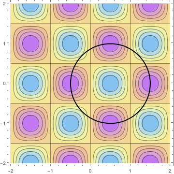
We want to understand the extrema of the function whose contours are plotted above, but only along the curve \(g(x,y) = 3\) (in black). Switching to the \(z = f(x,y)\) surface plot perspective, we have:

ContourPlot3D[
  {
    z == Sin[Pi x] Cos[Pi y],
    4 x^2 + 4 y^2 - 4 x == 3
  },
  {x, -2, 2}, {y, -2, 2}, {z, -2, 2},
  ContourStyle -> {
    Opacity[0.6],
    Opacity[0]
  },
  BoundaryStyle -> {
    {1, 2} -> Thick,
    2 -> None
  },
  Mesh -> None
]

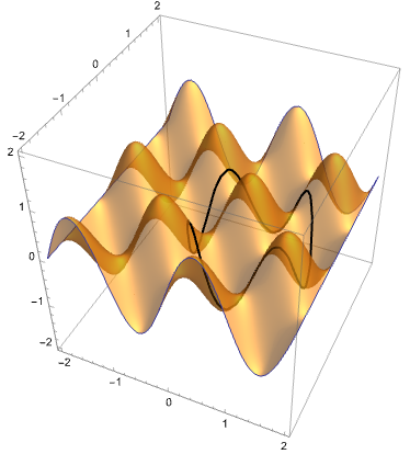
Using these plots, how can we visually identify the desired extrema?

Idea of Lagrange Multipliers

The system of \(f(x,y)\) constrained to \(g(x,y) = c\) will have an extreme value at \((x_0,y_0)\) if:

\(f(x,y)\) has an extreme value in its own right, or
The level curves of \(f\) and \(g\) are tangent at \((x_0,y_0)\).

Remember that level curves of a function are orthogonal to gradient vectors! In particular, the above conditions mean that

\(\nabla f(x_0,y_0) = 0\), or
\(\nabla f(x_0,y_0)\) and \(\nabla g(x_0,y_0)\) are parallel.

We can wrap these into a single equality (the Lagrange equations):

\[\nabla f = \lambda \nabla g \text{ for some } \lambda \in \mathbb{R}.\]

Values \((x_0,y_0,\lambda_0)\) satisfying this equation are called stationary points of the Lagrangian.

Example: \(f(x,y) = x^2 + 2 y^2\), \(g(x,y) = x^2 + y^2\), and \(c = 1\).

The stationary points of the Lagrangian are: \((-1, 0, 1), (1, 0, 1), (0,-1, 2), (0, 1, 2)\). The first two give minima of the system (\(f=1\)) and the last two give maxima (\(f=2\)).

Example: \(f(x,y) = x^4 + y^4 - 4 x y\), \(g(x,y) = x^2 + y^2\), and \(c = 2\).

The stationary points of the Lagrangian are: \((-1,-1, 0), (1, 1, 0), (-1, 1, 4), (1, -1, 4)\). The first two give minima of the system (\(f=-2\)) and the last two give maxima (\(f=6\)). What is the significance of the stationary points where \(\lambda = 0\)?